Solver Max - Taking a dip in the MIP solution pool

21 February 2022

Solution pool

We're frequently asked questions like: "How many other optimal solutions exist?" and "How do I find those solutions?". Often these questions are prompted by our mentioning that most models have alternative optima – that is, optimal solutions with the same objective function value, but different variable values.

Although a model may have a unique optimal solution, models with integer/binary variables typically have multiple optimal solutions, and continuous linear models may have an infinite number of alternative optimal solutions. The likely existence of multiple alternative optima is why we usually say "an optimal solution", rather than saying "the optimal solution".

Sometimes people also ask, "How do I find solutions that are almost optimal?". This question typically indicates that the decision maker may accept a sub-optimal solution (or an alternative optimal solution) that is "better" according to some criteria that aren't captured by the model design. Of course, we should look at incorporating the unspecified criteria within the model, but sometimes that is difficult or even impossible. In any case, exploring the solution space around the optimal solution is an important part of the modelling process.

This article describes methods for finding alternative optima and solutions that are almost optimal. Specifically, we explore the CPLEX "solution pool" feature, which NEOS Server has recently made available through their online portal.

Download the model

The model is available on GitHub.

Situation

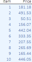
We have a list of items, each of which has a price. Part of the list is shown in Figure 1. In total, there are 30 items in this example.

We also have a target total price, representing the sum of some unknown number of items. Our objective is to select items such that the sum of their prices is as close as possible to the target total price – ideally, exactly matching the target total price.

This is an example of a class of problems known as the "subset sum problem". A typical situation where this type of problem might occur is when an accountant has a list of transactions and multiple invoices. However, the accountant doesn't know which transactions belong to a specific invoice, because the invoices are not itemized. We can use this model to match items to an invoice.

Model 1

Design: Model 1

Model formulation

Our model formulation is shown in Figure 2.

That is:

Equation (1). We want to minimize the absolute difference between the selected total price and the target total price (linearized).
Equation (2). The difference must be less than or equal to an upper bound (negative of the lower bound variable).
Equation (3). The difference must be greater than or equal to a lower bound variable.

Figure 2. Mathematical formulation for Model 1

\begin{alignat*}{1} &\text{Objective} \\ & \quad \text{Min } fAbsDiff \quad &= &\quad -vLB \tag{1} \\ \\ &\text{Subject to} \\ & \quad -vLB \quad &\ge &\quad \text{dTarget} - \sum_{i=1}^n \text{dPrices}_{i} \times vSelection_{i} \tag{2} \\ & \quad vLB \quad &\le &\quad \text{dTarget} - \sum_{i=1}^n \text{dPrices}_{i} \times vSelection_{i} \tag{3} \\ \\ &\text{Variables} \\ & \quad vLB &= &\quad \text{Difference lower bound, \$} \tag{4} \\ & \quad vSelection_{i} &= &\quad \begin{cases} 1, &\text{if item $i$ is selected} \\ 0, &\text{otherwise} \tag{5} \end{cases} \quad &\forall \ i \in I \\ \\ &\text{Data} \\ & \quad \text{dTarget} &= &\quad \text{Total target price, \$} \tag{6} \\ & \quad \text{dPrices}_{i} &= &\quad \text{Item prices, \$} \quad &\forall \ i \in I \tag{7}\\ \\ &\text{Sets} \\ & \quad I &\ &\quad \text{Item} \tag{8} \\ \\ &\text{Dimensions} \\ & \quad n &\ &\quad \text{Number of items} \tag{9} \\ \\ &\text{Bounds} \\ & \quad \text{Free} &\ &\quad \tag{10} \\ \end{alignat*}

Implementation

Select items

We use binary variables to represent the selection of each item. Then we calculate the difference between the target and the selected total price.

Figure 3 shows an example of a solution where the solver didn't find an exact match between the target total price and the total price of the selected items.

Our objective is to minimize the absolute value (linearized) of that difference. Ideally, the difference should be zero – though we need to allow for the possibility that no combination of the items exactly matches the target.

Note that the smallest difference could be positive or negative, so we need to specify both lower and upper bounds (which are symmetrical, for convenience, as only one of these constraints can apply at any time). In addition, the lower bound can be negative, so we specify the variable bounds as Free (rather than being restricted to being non-negative).

Solver model

Objective function

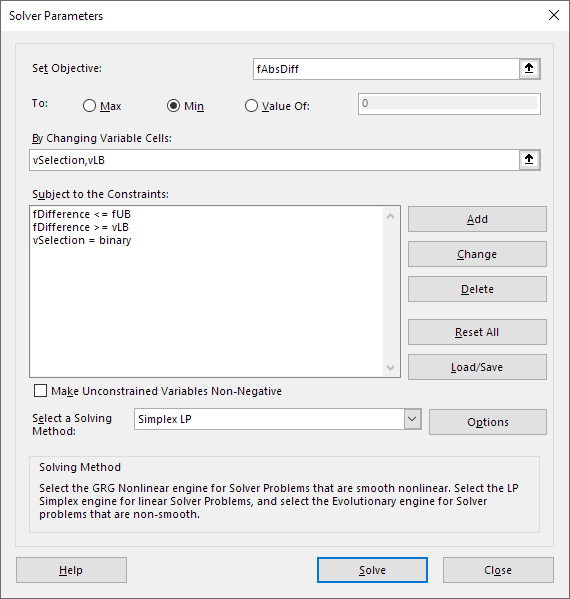
The Solver model is shown in Figure 4. Our objective is to minimize fAbsDiff.

Variables

The model has two sets of variables:

vSelection. Which items are selected from the list.
vLB. Lower bound of the total price difference.

Constraints

The constraints are:

fDifference <= fUB. The difference must be no more than the upper bound (negative of lower bound).
fDifference >= vLB. The difference must be at least the lower bound.
vSelection = binary. Selection variables are binary.

Note that the non-negativity option has been unselected.

Solution method

Our model is a mixed integer linear program that can be solved via either Solver or OpenSolver, though OpenSolver is much faster.

Analysis

Optimal solution

When we solve the model, OpenSolver finds an optimal solution that exactly matches the target total price, as shown in Figure 5. The lower and upper bounds on the difference are both zero, and consequently the absolute difference is also zero.

The solution is what we want, so all is good. However, as we mentioned earlier, most MIP models have multiple alternative optima. So, is that the case with this model?

Methods for finding alternative optima

Two methods for finding alternative optima are:

CPLEX solution pool. Use the CPLEX "solution pool" feature to find alternative solutions.
Eliminate known solutions. Add a constraint that excludes known solutions (optimal or otherwise).

We'll look at each of these methods in turn.

CPLEX solution pool

Thanks to NEOS Server

As an aside, we were recently working on a model where we thought that the solution pool feature might be useful.

The model was solved using CPLEX via the NEOS Server service. However, even though CPLEX generated the solution pool results, they were not available through the NEOS online portal.

After we asked NEOS about how to access the solution pool results, they amended their portal to provide the pool results in addition to the primary solution. We thank NEOS for making the change, along with their continued excellent service.

The CPLEX solution pool is a method for the solver to generate and output multiple solutions to a mixed integer programming (MIP) model. It can be used to output multiple alternative optima, along with other solutions that the solver finds either during or after the initial solution process.

We access CPLEX via the NEOS Server service, using a process like that described in our earlier article We need more power: NEOS Server.

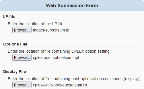
Generating the solution pool is straightforward. Having chosen to submit a CPLEX LP job via the NEOS online portal, we specify the LP file as usual, and then also specify a "Display File" that contains the following two lines:


    populate
    write pool.sol all

The first line instructs CPLEX to populate the solution pool, while the second line writes all pool solutions to a file called "pool.sol".

When we run CPLEX, NEOS returns a zip file that contains the pool.sol file and, if we selected the "Return .sol file" option, a soln.sol file that contains the incumbent optimal solution found by CPLEX. Note that the incumbent solution is also listed at the top of the pool.sol file (before the pool solutions).

In this case, CPLEX returns a pool of 58 solutions. After examining the file, we see that the pool contains two optimal solutions (i.e., our objective function value equals zero) – confirming that our model has multiple alternative optima. However, some of the pool solutions are very far from optimal, so the results have somewhat mixed usefulness.

Fortunately, we can control the pool generation process via a set of options, specified via "Options File" on the portal's form. For details of the options, see the CPLEX solution pool documentation.

Let's try some options, to see if we can improve the pool. First, we expand the scope of the pool by raising the pool "intensity" to its maximum setting:


    set mip pool intensity 4

The pool now contains 1856 solutions, which is many more than we want. We note that the pool still contains two optimal solutions. So, next we specify an option to reduce the "capacity" of the pool to return only 20 solutions:


    set mip pool intensity 4
    set mip pool capacity 20

The pool now has only 20 solutions, which is more manageable. The CPLEX log says "462 replaced", which indicates that it replaced solutions in the pool to fit the restricted capacity we specified. We can control the replacement process, specifically to prefer good solutions, by adding another setting:


    set mip pool intensity 4
    set mip pool capacity 20
    set mip pool replace 1

The pool now contains 20 solutions, all of which are very good solutions. However, there is only one optimal solution in the pool, so we've lost the other optimal solution found previously. By specifying the absolute gap between the pool solutions and the incumbent optimal solution, we can further control the quality of the pool solutions:


    set mip pool intensity 4
    set mip pool capacity 20
    set mip pool replace 1
    set mip pool absgap 0

That is, we specified an absolute gap of zero, meaning that the pool should be populated only with optimal solutions. The pool file now contains only five solutions, all of which are optimal. Note that the pool is not guaranteed to contain all optimal solutions. Finding all optimal solutions is, in general, a much more difficult problem than solving the model to find just an optimal solution. Nonetheless, CPLEX usually does a good job of finding alternative optima.

We can also populate the pool with solutions that are close to optimal. For example, if we set the absolute gap to be 0.015, rather than zero, then effectively we're asking CPLEX to find solutions within ±1 cent of optimal. Note that we specify 0.015, rather than 0.01, to allow for precision errors in the objective function, which has values like 0.0099999999998985345 and 0.010000000000012221 in the pool's solutions. If we set the absolute gap to be 0.01, then the latter solution would not be included in the pool.

Our final options file contains the lines:


    set mip pool intensity 4
    set mip pool capacity 20
    set mip pool replace 1
    set mip pool absgap 0.015

The resulting pool file contains 20 solutions, five of which are optimal, and the remainder are all ±1 cent from optimal. Inspecting these solutions provides an opportunity for us to identify solutions that we may prefer in favour of the incumbent optimal solution.

The three files we submitted to NEOS are available for download from near the top of this article. The NEOS job submission form, showing where each of the files is specified, is shown in Figure 6.

Eliminate known solutions

Figure 7. Result with optimal solutions eliminated

The second method for finding alternative optima is to eliminate known solutions by specifying a constraint that says the solutions are not feasible.

With the CPLEX solution pool having found five alternative optima, we've added a constraint to the model that excludes those solutions. This is, for each of the five solutions, we constrain the sum of the selection variables that equal 1 in the solution to be one less than the number of items selected in that solution.

For example, if we have an optimal solution in which the six items 7, 9, 14, 23, 27, and 29 are selected, then specifying that the sum of the variables for those items must be less than or equal to five prevents the solver from selecting that combination of items. Importantly, the constraint does not prevent the solver from finding a solution that selects five of those items plus one or more other items.

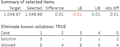
We have implemented this constraint in the example Excel file. The constraint includes an assumption called dEliminate, which switches this constraint on/off. With the switch set to TRUE, the result of running OpenSolver is shown in Figure 7. With the five known optimal solutions excluded, the optimal solution has a difference of 1 cent. Since the optimal solution is now worse than the optima we found previously, this result proves that there are only five alternative optima in this example.

If we didn't have the solution pool results, then we could incrementally eliminate solutions. That is, define the elimination constraint to exclude only the incumbent optimal solution and then re-solve the model. The result would be an alternative optima, which we add to the elimination constraint. We repeat this process until, on the sixth iteration, the solver returns a sub-optimal solution. At that point, we know that we have found all the model's alternative optima.

Conclusion

This article demonstrates use of the CPLEX solution pool feature, along with a process for excluding known solutions using a constraint. These methods for finding alternative optima can be very useful for exploring the solution space, enabling us to better understand the model and its solutions.

If you would like to know more about this model, or you want help with your own models, then please contact us.

Taking a dip in the MIP solution pool