3 April 2022

When formulating a model, we often have a situation described in terms of logic conditions where something implies something else. For example:
- If this happens, then we must do that.
- If this and that happen, then we can't do some other thing.
- We can do some or all of these things, but only if that other thing happens.
However, mathematical programming models cannot represent logic conditions directly. Therefore, we need to translate the conditions, known as "implications", into a set of constraints that represent the logic.
This article describes a technique for converting a logical implication into an equivalent set of constraints. Along the way, we'll dabble in applying some formal logic notation, define rules for manipulating formal logical implications, have a brief look at Conjunctive Normal Form (CNF), and learn how to convert CNF into constraints.
Part 2 describes an alternative representation of this technique, specifically designed to improve the proficiency of students learning to formulate models.
Download the model
The model is available on GitHub.
Situation
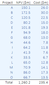
We have a list of 15 potential projects that we can do this year. As shown in Figure 1, each project has an initial cost and a Net Present Value (NPV), with the initial cost included in the NPV. We list the initial costs separately because we have a limited budget of $100m for initial cost expenditure this year, so we cannot do all projects.
Our objective is to select the projects that maximize the total NPV, subject to meeting the budget constraint.
We note that Projects A and B are the largest, in terms of initial cost and NPV. In addition, Projects C, D, and E partially overlap the scope of Projects A and B. If we do both A and B, then we cannot do any of C, D, and E. That is, we have a constraint on the combinations of projects that are allowed.
Model 1
Formulation for Model 1
Our model formulation is shown in Figure 2.
That is:
- Equation (1). We want to maximize the NPV of selected projects.
- Equation (2). Provided the initial cost of selected projects is within the budget.
- Equation (3). Placeholder for the project combinations constraint – which we'll add later.
Implementation
Apart from the project combinations constraint, which we'll add in Model 2, the model is simple.
That is, we use binary variables to represent the selection of each project. Then we calculate the total selected NPV and initial cost, for use in the objective function and budget constraint respectively.
Solver model
Objective function
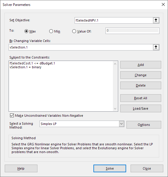
The Solver model is shown in Figure 3. Our objective is to maximize fSelectedNPV.1.
Variables
The model has one set of variables:
vSelection.1. Which projects are selected from the list.
Constraints
The constraints are:
fSelectedCost.1 <= dBudget.1. The total initial cost must be no more than the budget.vSelection.1 = binary. Selection variables are binary.
Solution method
Our model is a mixed integer linear program that can be solved via either Solver or OpenSolver.
Analysis
Optimal solution for Model 1
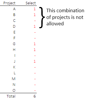
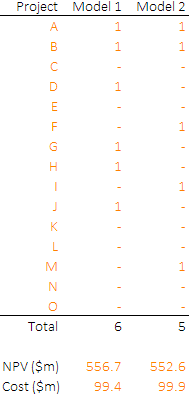
When we solve the model, OpenSolver finds an optimal solution that selects 6 of the 15 potential projects, as shown in Figure 4. The selection includes both Projects A and B, along with D, G, H, and J; producing a total NPV of $556.7m. The total initial cost is just under the budget, at $99.4m.
But we failed to meet our project combinations requirement
Our project combinations requirement says that we can't select any of Projects C, D, and E if we do both A and B. Since the model selected A, B, and D, this is not a valid solution – though the model doesn't know that, as we didn't tell it this requirement.
Therefore, we need to include a constraint that prevents this combination. We could add a manual constraint that prevents this specific solution, and then hope the next solution is valid (in terms of our currently implicit project combinations requirement), or keep adding manual constraints until we get a satisfactory solution.
Instead, let's explore a general technique for formulating this type of logic condition. Once we've described the technique we'll return to the project example to illustrate the technique in action.
Formulating logic conditions as constraints
From English to math
To convert a logic condition into a constraint, we need to:
- Understand the fundamental relationship between binary variables and Boolean values.
- Define some notation for expressing our logic condition formally.
- Specify some rules for manipulating formal logic conditions.
- Define Conjunctive Normal Form (CNF) as a specific way of expressing logic conditions.
- Convert a CNF expression into constraints.
These steps are outlined in the following sections. Note that some of this description is based on the document From English to math in 3 steps: A quick guide to writing logical expressions on binary variables as linear inequalities by Professor Tallys Yunes. That document explains the process in more detail and includes additional examples.
Binary variable = Boolean value
Fundamental to our approach is that our model uses Binary variables to represent Boolean logic values.
That is, 1 represents TRUE and 0 represents FALSE. For example, for each project \(p\), each of our project selection variables \(vSelection_p\) equals 1 if a project is selected (TRUE) or 0 if it is not selected (FALSE).
In addition, we can negate a Boolean value by subtracting it from 1. That is, if a Boolean is TRUE, then 1 - TRUE = FALSE, since 1 - 1 = 0. Similarly, if a Boolean is FALSE, then 1 - FALSE = TRUE, since 1 - 0 = 1.
Formal logic operators
Expression of formal logic conditions is a large and complex topic. But, for our purpose, we need to consider only the following operators:
- AND, represented by \(\land\)
- OR, represented by \(\lor\)
- XOR, represented by \(\oplus\)
- NOT, represented by \(\lnot\)
- IMPLIES, represented by \(\implies\)
- IFF (if and only if), represented by \(\iff\)
Note the difference between OR and XOR: OR (inclusive or) is true if at least one of the operands is true; XOR (exclusive or) is true if exactly one of the operands is true.
Rules for manipulating formal logic conditions
There are several rules that are useful for manipulating logic conditions:
- Rule 1: \(\lnot\)(\(\lnot\)x) = x
- Rule 2: \(\lnot\)(x\(\lor\)y) = \(\lnot\)x\(\land\)\(\lnot\)y
- Rule 3: \(\lnot\)(x\(\land\)y) = \(\lnot\)x\(\lor\)\(\lnot\)y
- Rule 4: x\(\land\)(y\(\lor\)z) = (x\(\land\)y)\(\lor\)(x\(\land\)z)
- Rule 5: x\(\lor\)(y\(\land\)z) = (x\(\lor\)y)\(\land\)(x\(\lor\)z)
- Rule 6: x\(\oplus\)y = (\(\lnot\)x\(\land\)y)\(\lor\)(x\(\land\)\(\lnot\)y)
- Rule 7: x\(\implies\)y = \(\lnot\)x\(\lor\)y
- Rule 8: x\(\iff\)y = (x\(\implies\)y)\(\land\)(y\(\implies\)x)
Note that IMPLIES and IFF have the highest (equal) priority, followed by NOT, AND, then OR. For example, \(\lnot\)x\(\land\)\(\lnot\)y means (NOT x) AND (NOT y).
Conjunctive Normal Form
Key to converting a logical implication into a constraint is expressing the expression in what is known as "Conjunctive Normal Form" (CNF). That is:
- The condition involves only some or all of the AND, OR, and NOT operators.
- A NOT operator can be applied only to a single term, rather than a group of terms.
- A group of terms uses only OR operators (where a term may include a NOT operator).
- Groups of terms use only AND operators.
For example, from the CNF Wikipedia page, (A\(\lor\)\(\lnot\)B\(\lor\)\(\lnot\)C)\(\land\)(\(\lnot\)D\(\lor\)E\(\lor\)F) is in CNF. It consists of two groups separated by an AND operator. Within each group, the terms are separated only by OR operators, with some terms within a group using a NOT operator.
Conversely, \(\lnot\)(B\(\lor\)C) is not in CNF, since the NOT operator is applied to a group rather than to a single term. We can convert the condition into CNF using Rule 2, producing \(\lnot\)B\(\land\)\(\lnot\)C.
Convert CNF into a constraint
Once a logic condition is expressed in CNF, we can apply the following steps to convert it into a constraint (or, often, a set of constraints):
- Step 1: Each group separated by \(\land\), or the whole group if there are no \(\land\) operators, becomes a constraint in the form "Group >= 1".
- Step 2: \(\lnot\) becomes "1-" (c.f. negating a Boolean value by subtracting it from 1).
- Step 3: \(\lor\) becomes "+".
Returning to our project selection example
Formal expression of our project combinations requirement
Our project combinations requirement is: If we do both A and B, then we cannot do any of C, D, and E.
In formal logic, the condition can be expressed as: (A and B) implies ((not C) and (not D) and (not E)).
Using the logic notation, this becomes: A \(\land\) B \(\implies\) \(\lnot\)C \(\land\) \(\lnot\)D \(\land\) \(\lnot\)E.
Derive CNF for our logic condition
Our logic condition is not in CNF because it uses an IMPLIES operator.
We can convert our logic condition to CNF using the rules for manipulating logic conditions. That is:
- Original condition: A \(\land\) B \(\implies\) \(\lnot\)C \(\land\) \(\lnot\)D \(\land\) \(\lnot\)E
- Apply Rule 7: \(\lnot\)(A \(\land\) B)\(\lor\) (\(\lnot\)C \(\land\) \(\lnot\)D \(\land\) \(\lnot\)E)
- Apply Rule 3: (\(\lnot\)A \(\lor\) \(\lnot\)B) \(\lor\) (\(\lnot\)C \(\land\) \(\lnot\)D \(\land\) \(\lnot\)E)
- Apply Rule 5: (\(\lnot\)A \(\lor\) \(\lnot\)B \(\lor\) \(\lnot\)C) \(\land\) (\(\lnot\)A \(\lor\) \(\lnot\)B \(\lor\) \(\lnot\)D) \(\land\)(\(\lnot\)A \(\lor\) \(\lnot\)B \(\lor\) \(\lnot\)E)
The last step converts our condition into CNF.
Use Wolfram|Alpha to convert into CNF
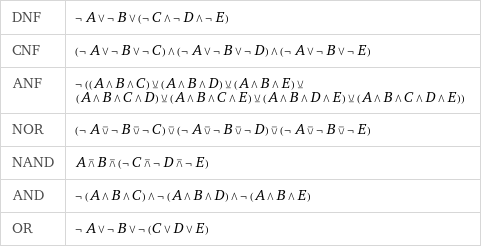
Applying the rules for manipulating logic conditions can be tricky. Fortunately, we can take a short-cut.
Wolfram|Alpha is a "computational knowledge engine and answer engine developed by Wolfram Research." (Wikipedia: Wolfram|Alpha). Amongst many other things, Wolfram|Alpha can manipulate mathematical expressions.
For example, we can give Wolfram|Alpha the following input, representing our logic condition:
(A and B) implies ((not C) and (not D) and (not E)).
As shown in Figure 5, the response from Wolfram|Alpha is a variety of equivalent logic expressions – including one in CNF. Wolfram|Alpha's CNF expression is the same as the CNF expression we derived above.
Convert our CNF into constraints
Now that we have a CNF expression, we can convert it into constraints using the process described above.
That is, we start with the CNF:
(\(\lnot\)A \(\lor\) \(\lnot\)B \(\lor\) \(\lnot\)C) \(\land\) (\(\lnot\)A \(\lor\) \(\lnot\)B \(\lor\) \(\lnot\)D) \(\land\) (\(\lnot\)A \(\lor\) \(\lnot\)B \(\lor\) \(\lnot\)E)
Step 1: Each group separated by \(\land\) becomes a constraint in the form "Group >= 1", so we create three constraints:
- (\(\lnot\)A \(\lor\) \(\lnot\)B \(\lor\) \(\lnot\)C) >= 1
- (\(\lnot\)A \(\lor\) \(\lnot\)B \(\lor\) \(\lnot\)D) >= 1
- (\(\lnot\)A \(\lor\) \(\lnot\)B \(\lor\) \(\lnot\)E) >= 1
Step 2: \(\lnot\) becomes "1-":
- (1-A) \(\lor\) (1-B) \(\lor\) (1-C) >= 1
- (1-A) \(\lor\) (1-B) \(\lor\) (1-D) >= 1
- (1-A) \(\lor\) (1-B) \(\lor\) (1-E) >= 1
Step 3: \(\lor\) becomes "+":
- (1-A) + (1-B) + (1-C) >= 1
- (1-A) + (1-B) + (1-D) >= 1
- (1-A) + (1-B) + (1-E) >= 1
Finally, with a bit of algebra left as an exercise for the student, these constraints can be rearranged and simplified to:
- A + B + C <= 2
- A + B + D <= 2
- A + B + E <= 2
Interpretation of constraints derived from logic conditions is often difficult. But in this example, the interpretation is straightforward.
The first constraint says that up to two of Projects A, B, and C can be selected. That is, remembering that each project is represented by a Binary variable where 1 means it is selected and 0 means it is not selected:
- If A and B are selected, then C cannot be selected (i.e. 1 + 1 + 0 <= 2).
- If A is selected and B is not selected, then C may be selected (though it does not have to be, as 1 + 0 + 0 <= 2 and 1 + 0 + 1 <= 2).
- If A is not selected and B is selected, then C may be selected (though it does not have to be, as 0 + 1 + 0 <= 2 and 0 + 1 + 1 <= 2).
- If A is not selected and B is not selected, then C may be selected (though it does not have to be, as 0 + 0 + 0 <= 2 and 0 + 0 + 1 <= 2).
Similarly for the other two constraints involving Projects D and E. Collectively, this set of constraints represent the logic condition that we are looking to implement.
Model 2
Formulation for Model 2: Add the logic constraints to Model 1
In Model 1 we left a placeholder, constraint (3), for the project combinations constraint. We're now ready to fill that placeholder.
Recall that our projects are numbered from n = 1 to 15, representing Projects A, B, C, ..., O. Therefore, the three constraints derived above can be represented as shown in Figure 6.
Optimal solution for Model 2
In the spreadsheet, the combination constraints for Model 2 are controlled via the "Combinations" drop-down list, which has two options:
- "Active". The combination constraints are applied with a RHS of 2, which restrict the allowed project combinations.
- "Inactive". The combination constraints are applied with a RHS of 4, which can never be binding, effectively making the project combinations unconstrained. Note that a RHS of 4 is chosen simply because it is large enough to make the constraint non-binding. We could use a RHS of 3, though that will sometimes bind, which might have unintended consequences. Any value larger than 4 would also work.
With the additional project combination constraints (3a, 3b, and 3c) active, the optimal solution for Model 2 is shown in Figure 7. The optimal solution for Model 1 is also shown, for comparison.
When we solve Model 2, OpenSolver finds an optimal solution that selects 5 of the 15 potential projects. The selection includes both Projects A and B, along with F, I, and M; producing a total NPV of $552.6m. The total initial cost is just under the budget, at $99.9m.
This solution uses slightly more of the available budget, but – as is expected when adding constraints – has a slightly lower objective function value (at best, the objective function value could be the same as for Model 1). The set of selected projects still includes Projects A and B, but otherwise it is entirely different.
Importantly, because both Projects A and B are selected, the solution includes none of Projects C, D, and E. That's what we were trying to achive with the project combinations constraint, though it turned out that we needed a set of constraints, rather than a single constraint, to implement the necessary logic condition.
Conclusion
This article demonstrates a technique for formulating logic conditions as constraints in a mathematical program. This technique is often needed when we are formulating a model.
Part 2 explores this topic further, including an alternative technique for converting logical implications into constraints, illustrated by several additional examples.
If you would like to know more about this model, or you want help with your own models, then please contact us.
References
The process for creating CNF expression and converting into constraints is described in:
Yunes, T. (2008). "From English to Math in 3 steps: A quick guide to writing logical expressions on binary variables as linear inequalities", Department of Management Science, University of Miami, pages 1 to 4.
