Jury simulation using SimPy

15 July 2025

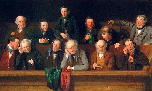
Following on from our previous article, Efficient jury empanelling: Respecting people's time, in this article we replicate the jury simulation model using the SimPy library.

SimPy is a process-based discrete-event simulation framework in Python. It is widely used for simulation of many and varied systems, especially those with queues, where time can be expressed in discrete steps.

Discrete-event simulation is often applied to the design, analysis, and improvement of complex systems such as factory production lines, transportation networks, and warehouses. A simulation model can help us identify critical components of a system and evaluate alternative designs, leading to improvements in performance and reductions in cost. That's exactly what we want to do.

Here we design and build Model 2, using SimPy to model the jury summoning process, with the goal of reducing the number of people needing to be summoned for jury service.

Download the model

The model described in this article is built in Python.

The files are available on GitHub.

Situation

As described in the previous article, Model 1 simulates the jury selection process for criminal trials in a Court. The process involves summoning (requiring people to attend) and empanelling (where people may be chosen to serve on a jury).

In this article we have the same situation, except that we use the SimPy library to implement the simulation as Model 2.

A brief overview of SimPy features

SimPy provides a set of features to help us build and manage a simulation model. In the jury situation, the main features we use are:

• Environment. Creates the core simulation environment that manages the simulation clock and event scheduling. Used via self.env = simpy.Environment() in the Model class, to represent the Court.
• Resources. Court staff are a limited resource. We assume that there is only one staff member and that they can handle only one task at a time. This is a convenient though not important assumption. A resource with capacity of one is created with self.staff = simpy.Resource(self.env, capacity=1). Resources are used with context managers like with self.staff.request() as req: to handle staff interactions with potential jurors. If the availability of Judges is an important aspect to consider, then we could also have a Judge resource. However, that's outside our scope so we just use the staff resource for all roles.
• Containers. We model the jury box in a courtroom as a container to be filled with jurors. The containers are created like self.jury_box = [simpy.Container(self.env, init = 0, capacity = gbl.required_jurors_per_trial)]. Each container is initially empty and has a capacity matching the required number of jurors. Jurors are empanelled using a put(1) operation and the jury box is tracked via a container's level and capacity.
• Processes. We use env.process() to create and manage multiple processes that may occur concurrently. Key processes include juror generation, summoning, excuse handling, show-up processing, and empanelment.
• Time management. The model uses statements like yield self.env.timeout() throughout to simulate time passing. This models various delays like response times, processing times, and gaps between events. Time is measured in minutes as the base unit, with the current simulation time being self.env.now. Most functions use the Python yield statement to pass control to another function while a function waits until it needs to run. The function may resume running from the yield point at a later time. This differs from the return statement that usually marks an exit point of a Python function.
• Resource queuing. We use SimPy's built-in queuing system through the Resource class. Jurors must wait for staff availability when requesting service. SimPy automatically manages contention for limited staff resources.

This combination of features allows the simulation to model complex interactions between multiple jurors, staff, and courtrooms while maintaining proper timing and handling resource constraints.

SimPy model structure

The best guide we've seen for how to design and build SimPy models is provided by Health Service Modelling Associates (HSMA). Their Little book of discrete-event simulation and Introduction to Discrete Event Simulation with SimPy video training series (2A, 2B, and 2C) are excellent. If you want an introduction to SimPy, then the HSMA material is a great place to start.

HSMA recommend an object-oriented structure for building models with SimPy. While that structure isn't the only way to organize a SimPy model, it provides a consistent, maintainable pattern that makes it easier to modify and share models between developers. Therefore, we broadly follow the recommended structure in our jury model.

The structure, as shown in Figure 2, has four main types of classes: gbl (for global values), entities, model, and simulation.

Implementation

Key details

We replicate the summoning and empanelling process described in the previous article. The main difference is that Model 1 takes an aggregated view of the process, because it isn't too concerned with the individual experience of participants. Conversely, the SimPy Model 2 explicitly represents each step that each participant goes through during the summoning and empanelling process.

A fundamental decision for a SimPy model is the time unit. In our jury situation, the selection and summoning of jury candidates takes place six week before the empanelling steps, which occur over a few hours or days. SimPy time units are real numbers, rather than integers, so we don't need to worry too much about precision. Nonetheless, it is best to choose a time unit that represents the smallest useful time unit in the model's situation. In our case, we choose a time unit of minutes.

Note that SimPy models only the discrete times when events occur, rather than stepping through every minute of the time period. For example, after jury candidates are summoned and potentially excused from service, there may be weeks in which nothing happens before the empanelling process begins. SimPy skips over the time periods in which no events occur.

In the model, it is important that all times are expressed in the same time unit. To account for periods of days and week in our model, using a base unit of minutes, we define time conversion constants for elasped_day and elasped_week. As show in Figure 3, these constants are used to represent time periods like the 8 week duration of the simulation.

    # Time constants
    elapsed_day = 60 * 8  # Minutes per day
    elapsed_week = elapsed_day * 5  # Minutes per week

    # Process timing. Base time unit is minutes
    trial_week = 6 * elapsed_week  # Start of trial week
    reporting_time = 7 * elapsed_week  # Start of final reporting on trial outcomes
    duration = 8 * elapsed_week  # End time for the simulation

Length of Python code in Model 2 compared with Model 1

The Python code for Model 1, which is written without using a simulation library, is 274 lines long. The Python code for Model 2 is 433 lines long. The main reason why the SimPy model has more code is that it details the timing of every step for every participant in the process, whereas Model 1 operates at a more aggregated level.

In other situations, a SimPy model may be shorter than an equivalent model written without a simulation library. The length and complexity of the code depends on many factors. For our purpose in writing Model 1, we didn't need to focus on the fine details of when events happen to each individual in the system. Where that type of focus is necessary or useful, using a library like SimPy can be very beneficial.

We won't go through all of Model 2's code in detail. It is available on GitHub if you want to examine the code or play with the model.

Essence of the SimPy model

The essence of how Model 2 works is captured in the three functions shown in Figure 4, all of which are in the Model class. That is:

• The assign_generate function generates each of the people assigned to a jury. Each simulated person has attributes like a unique identifier and the trial that they may be assigned to. After creating a candidate, this function calls the assign_process function. In many SimPy models, a generator function runs throughout the whole simulation time. In our model, the generator functions create a defined number of people only at the start of the simulation.
• The assign_process function represents the steps each assigned jury candidate goes through, specifically: summon, response, excuse by staff, show at Court, and the empanelling process.
• The assign_summon function, for example, summons each assigned jury candidate. First there is a queue while the process waits for the staff member to be available, then the summoning process takes some time, after which the candidate is designated as assigned.summoned = True.

    def assign_generate(self, num_trials):  # Generate each assigned person
        yield self.env.timeout(gbl.assign_generate - self.env.now)  # Start of process
        self.num_assigned = num_trials * gbl.assigned_jurors_per_trial
        self.results['a_initial'] += self.num_assigned
        curr_trial = 0
        for j in range(self.num_assigned):
            if j % gbl.assigned_jurors_per_trial == 0:
                curr_trial += 1
            self.assigned_counter += 1
            assigned = Assigned_Juror(self.assigned_counter)
            assigned.trial = curr_trial
            logger.debug(f'Assigned {assigned.id:>4,} for trial {assigned.trial} created at {self.env.now:>8,.1f} ({convert_time(self.env.now, 'days')})')
            self.env.process(self.assign_process(assigned, num_trials))
            yield self.env.timeout(0)

    def assign_process(self, assigned, num_trials):  # Process each assigned person
        yield self.env.timeout(gbl.assign_summon - self.env.now)  # Advance clock to summon process
        self.env.process(self.assign_summon(assigned))
        yield self.env.timeout(gbl.assign_response - self.env.now)  # Advance clock to responses
        self.env.process(self.assign_staff_excuse(assigned))
        yield self.env.timeout(gbl.trial_week - self.env.now)  # Advance clock to trial week
        self.env.process(self.assign_show(assigned))
        yield self.env.timeout(gbl.trial_week + gbl.show_cutoff + gbl.assign_empanel_gap - self.env.now)  # Advance clock to empanelling time
        self.env.process(self.assign_empanel(assigned, num_trials))

    def assign_summon(self, assigned):
        summon_time = random.expovariate(1.0 / gbl.assigned_mean_summon_time)
        yield self.env.timeout(summon_time)
        with self.staff.request() as req:  # Summon each assigned person, if not already challenged
            yield req
            start = self.env.now
            process_time = np.random.lognormal(mean=1.0, sigma=0.5)
            end = start + process_time
            assigned.summoned = True
            logger.debug(f'Assigned {assigned.id:>4,} summoned at {start:>8,.1f}, took {process_time:>8,.1f}, end at {end:>8,.1f} ({convert_time(end, 'days')})')
            yield self.env.timeout(process_time)

Each of the other process steps has a function like the assign_summon function. Although the code is quite long, an advantage of the recomended HSMA structure is that code can be organized in a way that is logical and easy to understand. There are similar functions for the pool of unassigned people, differing only in the details of how the two types of people proceed through the system.

Managing the iteration process in the simulation

The other key part of the model is that we need to run the process many times to get a good sample of behaviour. That's especially important in the jury situation, because we want to get accurate estimates of how often rare events occur, particularly a trial failing because we have insufficient candidates to empanel a jury.

The iteration process is managed by the Simulation class, including the central run_simulation function shown in Figure 5. This function calls the Model class to run each iteration, collating statistics from each iteration along the way.

We typically run the simulation for 100,000 or 1,000,000 iterations, to get good samples of the statistics. Note that Model 2 takes about 50 times longer to run than Model 1. That's because the SimPy model is operating at a much finer level of detail.

    def run_simulation(self):
        for iteration_number in range(1, gbl.num_iterations+1):
            logger.debug(f'\nIteration {iteration_number}')  # Print iteration when debugging
            if iteration_number % gbl.iteration_update == 0:
                print(f'Iteration: {iteration_number:,.0f}')  # Print iteration when in batch mode
            sim_model = Model(iteration_number)
            results = sim_model.iteration()
            self.collate_results(iteration_number, results)

Debug mode

Like Model 1, we've included debug statements in Model 2. To use debug mode, set num_iterations = 1 (or no more than a few iterations) and log_level = 'debug'. The model will print a line of output for each event that happens to each assigned and pool person. Each event occurs at a specific time and may have an associated duration.

An example of the debugging output is shown in Figure 6. To keep the output short, we've set pool_jurors_per_trial = 3, pool_min = 5, and assigned_jurors_per_trial = 8. These parameters are almost certainly inadequate to form a jury in the one trial scheduled in this iteration so, unsurprisingly, this run fails to empanel a jury.

DEBUG: Generated 1 trial for the scheduled week
DEBUG: Assigned    1 for trial 1 created at      0.0 (0.00 days)
DEBUG: Assigned    2 for trial 1 created at      0.0 (0.00 days)
DEBUG: Assigned    3 for trial 1 created at      0.0 (0.00 days)
DEBUG: Assigned    4 for trial 1 created at      0.0 (0.00 days)
DEBUG: Assigned    5 for trial 1 created at      0.0 (0.00 days)
DEBUG: Assigned    6 for trial 1 created at      0.0 (0.00 days)
DEBUG: Assigned    7 for trial 1 created at      0.0 (0.00 days)
DEBUG: Assigned    8 for trial 1 created at      0.0 (0.00 days)
DEBUG: Pool        9 created at    480.0 (1.00 days)
DEBUG: Pool       10 created at    480.0 (1.00 days)
DEBUG: Pool       11 created at    480.0 (1.00 days)
DEBUG: Pool       12 created at    480.0 (1.00 days)
DEBUG: Pool       13 created at    480.0 (1.00 days)
DEBUG: Pool       12 summoned at    960.2, took      2.4, end at    962.6 (2.01 days)
DEBUG: Pool       10 summoned at    962.6, took      3.0, end at    965.6 (2.01 days)
DEBUG: Pool        9 summoned at    965.6, took      4.4, end at    970.0 (2.02 days)
DEBUG: Pool       11 summoned at    970.0, took      2.4, end at    972.4 (2.03 days)
DEBUG: Pool       13 summoned at    972.4, took      2.6, end at    975.0 (2.03 days)
DEBUG: Assigned    8 summoned at  1,440.0, took      7.4, end at  1,447.4 (3.02 days)
DEBUG: Assigned    7 summoned at  1,447.4, took      3.1, end at  1,450.5 (3.02 days)
DEBUG: Assigned    6 summoned at  1,450.5, took      3.8, end at  1,454.3 (3.03 days)
DEBUG: Assigned    5 summoned at  1,454.3, took      3.3, end at  1,457.6 (3.04 days)
DEBUG: Assigned    2 summoned at  1,457.6, took      3.7, end at  1,461.3 (3.04 days)
DEBUG: Assigned    1 summoned at  1,461.3, took      2.4, end at  1,463.7 (3.05 days)
DEBUG: Assigned    3 summoned at  1,463.7, took      7.9, end at  1,471.7 (3.07 days)
DEBUG: Assigned    4 summoned at  1,471.7, took      3.8, end at  1,475.4 (3.07 days)
DEBUG: Assigned    4 excused by staff at  7,200.2 (15.00 days)
DEBUG: Pool       11 responded at  7,200.9 (15.00 days)
DEBUG: Pool       12 responded at  7,201.3 (15.00 days)
DEBUG: Pool        9 responded at  7,201.5 (15.00 days)
DEBUG: Pool       13 responded at  7,206.0 (15.01 days)
DEBUG: Pool       13 excused by staff at  7,206.0 (15.01 days)
DEBUG: Pool       10 responded at  7,206.5 (15.01 days)
DEBUG: Pool       12 showed up at 14,406.5
DEBUG: Pool       10 showed up at 14,407.5
DEBUG: Assigned    1 showed up at 14,407.7
DEBUG: Pool       11 showed up at 14,408.6
DEBUG: Assigned    7 showed up at 14,411.9
DEBUG: Pool        9 showed up at 14,415.2
DEBUG: Assigned    6 showed up at 14,424.9
DEBUG: Assigned    3 showed up at 14,428.7
DEBUG: Assigned    6 empanelled at 14,520.7 on trial 1 which has  1 jurors
DEBUG: Assigned    1 empanelled at 14,528.0 on trial 1 which has  2 jurors
DEBUG: Assigned    7 empanelled at 14,541.1 on trial 1 which has  3 jurors
DEBUG: Assigned    3 empanelled at 14,578.1 on trial 1 which has  4 jurors
DEBUG: Pool        9 challenged by lawyer at 14,580.6 (30.38 days)
DEBUG: Pool       12 empanelled at 14,582.0 on trial 1 which has  5 jurors
DEBUG: Pool       10 excused by Judge at 14,584.5 (30.38 days)
DEBUG: Pool       11 empanelled at 14,592.4 on trial 1 which has  6 jurors
DEBUG: Trial 1 status: fail

Initial results

Replicate the scenarios from Model 1

Figure 7 shows a summary of the scenario results from Model 1. Scenario 4 provides an 83% reduction in the number of people we need to summon who are not empanelled on a jury (the "extra" people), with only a small increase in the risk of failing to empanel a jury. Scenario 5 offers a slightly lower reduction in the number of people, while having a substantially lower risk of failing compared with the current system design.

Running the same scenarios in Model 2 produces the same results for the flow of people through the system (give or take small random sampling variations), but much higher risk of failure for each scenario – as shown in the last column of Figure 8. For Model 1, Scenarios 4 and 5 are great alternatives to the current system. But in the SimPy results, Scenarios 4 and 5 are no longer acceptable. These results are initially surprising, as the two models are intended to essentially represent the same process.

In simulation modelling, details matter

Many people assume that simulation is a simple method for modelling a system. But this view is misguided. In reality, simulation is often a difficult method. The key issue is calibrating a simulation model to match the real system. Getting a simulation that's realistic enough to be useful can be a very difficult and time-consuming task.

Of course, matching a model to the real world is also difficult for other modelling methods. For example, does my queuing system really have a Poisson arrival process with no baulking, as assumed by the queue equations? Even so, it is easier to gloss over the mismatch between model and real world with other methods, because they may deliver useful insights faster than a simulation can.

In this situation, our two models have different representations of the real system: Model 1 is aggregated, whereas Model 2 represents every individual going through every step of the process. The key point where the models differ is where people are excused from the jury process (either entirely, by staff after being summoned, or for a specific trial by a Judge). That is:

• Model 1 picks a sample from a Normal probability distribution, given a mean and standard deviation for the number of people to excuse. It then randomly selects that number of people to excuse.
• Model 2 takes a different approach, with each person having a probability of being excused. Importantly, Model's 2 probability of being excused is the same as the mean of the Normal distribution used in Model 1.

These two methods may not seem that different. But in simulation modelling, the details matter. Model 2's method is equivalent to a Binomial probability distribution (given a Bernoulli choice between being excused or not for an individual), rather than a Normal distribution (for the number of people being excused in aggregate).

To see how a different probability distribution can affect the results, Figure 9 shows sample and theoretical distributions for the number of people excused in Scenario 1, where we start with summoning 54 people, with a mean of 20% excused and, for the Normal distribution, a standard deviation of 5%. The data for these charts is produced by the distributions.py code in the GitHub repository.

The top (red) chart shows the result for Model 1, using a Normal distribution. The bottom (blue) chart shows the result for Model 2, using individual decisions (which equates to a Binomial theoretical distribution). In both models, the simulated and theoretical distributions are very similar, as we generally expect with a sample size of 1,000,000 iterations.

The Model 1 and Model 2 distributions are very similar. This is to be expected, as the number of people we start with (54) is reasonably large and the mean number of excused people is about 20% * 54 = 10.8. Model 2 has a slightly larger tail to the right, meaning that slightly more people will be excused and hence there's a higher risk of failing to fill a jury. Because the distributions are similar, the effect is relatively small – increasing the risk from 1 in 750 years for Model 1 to 1 in 244 years for Model 2.

But what if we start with a smaller number of people, like 20 – as we do for the number of assigned people in Scenario 4. The mean number of excused people is now about 20% * 20 = 4. Figure 10 shows the simulated and theoretical distributions for Model 1 (top) and Model 2 (bottom).

These distributions are materially different. In particular, the Model 2 distribution has a larger and longer tail to the right, meaning that Model 2 will excuse materially more people than Model 1 does. Having more excused people increases the risk of there being insufficient people to fill a jury. We see this in Figure 8 above, where Model 2 has a much higher risk of failure – expected to fail once every 8 months compared with 1 in 100 years for Model 1.

We note that the simulated Normal distribution also doesn't fit the theoretical distribution quite so well, due to rounding to a whole number of people and truncating the distribution at both zero and the number of available candidates in a specific iteration.

The small difference in how we model the excusing process leads to materially different results. This is a general lesson for simulation modelling: small differences can matter. In this situation, we have no data about what the probability distribution is and how many people are excused. In practice, we would need to gather data to make an informed decision about how to accurately model this aspect of the process.

Reconciling and validating the models

Having built two models of the jury process, it would be very useful to reconcile their results and validate the correctness of the models. This is an important topic in simulation modelling. Simulating a system is relatively easy. Validating that a simulation model accurately represents the system behaviour is hard.

One approach that addresses some validation and verification issues is to build two models – either using similar methods built by separate teams or using different methods (ideally built by separate teams). We've adopted the latter approach. But our models produce materially different results, so we need to reconcile them.

We've explained above one reason why the two models produce different results. Model 1 can easily be modified to use a Binomial distribution to select the number of people to excuse, rather than using a Normal distribution. Therefore, we've modified Model 1 to provide a choice of distributions. The code for making that choice is shown in Figure 11.

        mean = len(candidates) * mean_rate / 100
        stdev = mean * (stdev_rate / mean_rate)
        if REMOVE_DISTN == 'normal':  # Probability distribution for removing candidates
            num_removed = int(round(np.random.normal(mean, stdev), 0))  # Normal distribution
            num_removed = max(0, min(num_removed, len(candidates)))
        else:
            num_removed = np.random.binomial(len(candidates), mean_rate / 100, 1)[0]  # Binomial distribution

Figure 12 compares the failure rates for the models. There are significant differences between the Normal and Binomial distributions for Model 1, especially for Scenarios 4 and 5. The results for Model 1 using the Binomial distribution and Model 2 are similar. This similarity suggests that most of the difference between the models is due to the choice of how excuses are modelled, plus or minus some random variation due to the sampling process. There are other differences between the models, such as the handling of individuals empanelled on failed trials, but the impact of those differences is very small.

Final result

Which model is correct? We don't know, because we don't have sufficient data about the real system. But, all else being equal, we probably should use Model 2 (or Model 1 with a Binomial distribution), as it is more conservative – which is very important to the Courts and Judiciary.

If we do that, then to offset the higher failure rate in Model 2, we can simply increase the number of assigned people in Scenario 4 (which is our preferred scenario), leading to Scenario 6. Or we can do a grid search of parameters to find the best trade-off between risk and number of extra people, which is Scenario 7. These scenarios are summarized in Figure 13, along with the current situation. That is:

• Scenario 4: For Model 1 using a Normal distribution, Scenario 4 has a pool of 4 people per trial, minimum pool size of 17 people summoned, plus 20 people summoned to be assigned to a jury. These parameters lead to summoning 77 people, of whom 46 are expected to show. After empanelling 36 epople, we have 10 extra people. There is a 1 in 100 year risk of failure and an 83% reduction in the number of extra people needed for the jury process (10 vs 61 currently).
• Scenario 6: For Model 2 (or Model 1 with a Binomial distribution), to achieve a similar level of risk, we could keep the pool parameters the same and increase the number of people summoned to be assigned to a jury to 27. This leads to about a 1 in 100 year risk of failure and a 62% reduction in the number of extra people needed for the jury process.
• Scenario 7: Alternatively, for Model 2 (or Model 1 with a Binomial distribution), we could change the mix of pool and assigned people: summon a pool of 7 people per trial, minimum pool size of 21, and summon 23 people to be assigned to a jury. This leads to about a 1 in 100 year risk of failure and a 67% reduction in the number of extra people needed for the jury process.

So, the results for Scenarios 6 and 7 from Model 2 (or Model 1 with a Binomial distribution) are not quite as good as Scenario 4 from Model 1. Nonetheless, even with more conservative assumptions, our simulation modelling has shown that it is possible to achieve a substantial saving in extra people summoned for jury service, relative to the current system design, while having an acceptable risk of failure.

Conclusion

In this article, we describe a simulation model of the jury summoning and empanelling process for criminal trials in a Court, using the SimPy library.

The SimPy model operates at a finer level of detail compared with our previous aggregate model. Therefore, not surprisingly, the SimPy model is much slower.

But having a second model of the situation highlights an important detail relating to choice of probability distribution for one of the decisions in the jury process. Whether we model the excuse process using a Normal or a Binomial distribution makes a material difference to the results. We can reconcile the difference between the models by using either distribution in Model 1, with the choice of a Binomial distribution closely matching the results of Model 2. This illustrates a key lesson for simulation modelling in general: details matter, sometimes a lot.

Even with the more conservative results from Model 2, our proposed change to the jury service process (pre-assigning people to juries), reduces by about two-thirds the number of extra people who need to be summoned to Court. This change makes jury service more efficient, enabling it to meet the needs of the justice system while also respecting the time of people who participate.

If you would like to know more about this model, or you want help with your own models, then please contact us.