Solver Max - Pivot irrigators in a 100 acre field

3 April 2025

Most optimization models are linear for a very practical reason – linear models are easier to solve. Situations that involve non-linear relationships are often linearized, or approximated with linear relationships, for the same reason. But not all situations are easily linearized.

In this article, we explore a model for optimizing the layout of centre-pivot irrigation machines in a field. Our goal is to see if replacement of the existing worn-out machines would make purchase of a field a viable investment.

Pivot irrigators are commonly used by crop farmers to supplement natural rainfall. For example, large areas of the mid-west USA are covered with these machines, such as this part of Kansas. The machines are almost always arranged in a simple grid pattern, which is not an efficient design in terms of coverage.

Arranging pivot irrigators in a field is a type of circle packing problem, with a non-linear objective and non-linear constraints. Worse still, the model is non-convex. These characteristics make our optimization problem both difficult and interesting.

To solve our model, we try several free and commercial solvers. All fail to find good solutions, except in trivial cases. So we try another solver, MINLP-BB via NEOS Server, that finds locally optimal solutions with no guarantee of global optimality. But by using a multi-start technique, we improve our chances of finding a good, perhaps optimal, solution. Is that solution good enough to justify making an investment?

Download the models

The models described in this article are built in Python using the Pyomo library.

The files are available on GitHub.

Situation

Current installation — Figure 1. Current pivot irrigator installation

We're a farmer considering the purchase of a field in a semi-arid region. In this region, only irrigated areas are productive.

The field is rectangular, with sides in imperial units of 3,000 feet East-West by 22 chains North-South. That equates to 1,000 yards by 484 yards, for a total area of exactly 100 acres.

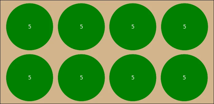
The current farmer delivers water to the field using pivot irrigators – that is, irrigation machines that have a fixed centre and rotate in a circular motion. The machines are worn out, so we need to replace them. As shown in Figure 1, the current installation has eight machines arranged in a regular pattern, as is the norm for pivot irrigation layout. Each machine consists of 5 x 20 metre segments (100 metre radius). Each machine irrigates an area of 31,416 square metres, for total coverage 251,327 square metres, which is 62.10% of the field's area.

To maximize crop yield, it is important that we irrigate as much of the area as possible. However, we need to account for the cost of the machines, along with the operational and maintenance costs over their lifetime.

Our questions are:

Is there a better arrangement of pivot irrigation machines in this field?
Should we purchase the field and install new machines?

Background on pivot irrigators

Figure 2. Everything about irrigation pivots

Some pivot irrigator systems are massive, with a radius of half a mile (about 800 metres), covering an area of about 500 acres (200 hectares). Our field is much smaller, being 100 acres in total area, so we are considering smaller machines – though the concept is the same.

Our field's boundaries were surveyed long before pivot irrigation machines were invented in the 1940s, so our field is not ideally sized for the machines that are available. This mismatch between the field's dimensions and the machines is common, though it makes the layout problem even more difficult.

The Smarter Every Day YouTube channel has a great video about the installation and operation of a centre-pivot irrigator, as shown in Figure 2. It is worth watching the video to understand the context of our situation.

Investment characteristics

We can replace the current pivot irrigators with machines of the same type. The characteristics of the potential investment are:

The field measures 1,000 yards by 484 yards, with a total area of exactly 100 acres. In metric units, the field is 914.400 by 442.570 metres, with a total area of 40.4686 hectares.
Each machine costs $36,000 to purchase and install. A machine consists of the pivot mechanism and a single 20 metre long built-in segment.
Additional 20 metre long segments can be purchased at a cost of $12,000 each. A machine may have up to a total of eight segments (including the built-in segment).
The machines are expected to have a 15 year life.
Each year, we expect to have maintenance costs of $1,000 for each machine's pivot and built-in segment, plus $500 per additional segment.
We have fixed operating costs of $180,000 per annum, covering costs for other machinery and staff associated with working the field.
The market price for purchasing the field is $640,000. This equates to $6,400 per acre, which is high for this type of land, but there are few other choices available in the region.
The planned crop will yield an average gross margin of $1.35 per square metre per year, allowing for all variable costs (planting, harvesting, etc).
Our real, weighted-average cost of capital (WACC) is 10% per annum.
The annual cashflows have a Net Present Value (NPV) multiplier of 7.6061. That is, $1 per annum for 15 years at a discount rate of 10% is worth $7.6061 NPV.

Figure 3 shows a calculation of the total investment value based on replicating the existing machine layout. Each of the machines produces an NPV of $215,767 allowing for the annual yield from the area they irrigate less their initial costs and annual costs. After deducting the cost of the field and the NPV of the annual fixed operating cost, the overall investment value is -$282,958.

That is, with a negative NPV, the investment is not worthwhile. But what if we can find a better layout?

Figure 3. Investment value of current layout (NPV)

Model design

Creating a better layout equates to choosing the number of machines, the number of segments, and the position of each machine in the field. This is a type of circle packing problem, where the radii of the circles are integers (number of segments for each machine, multiplied by the length of each segment). We want to maximize the overall NPV of our investment. A positive NPV would indicate that this is a worthwhile investment.

We need to ensure that the circles covered by each machine do not overlap, so the machines cannot collide as they rotate and the crop is not over-watered. The coverage circles must also be entirely within the field, so we don't trespass onto our neighbours' lands.

We can formulate the situation as a non-linear optimization model:

In the objective function, we deduct the various costs from the yield, discounting the cashflows to produce an NPV. Note that the NPV calculation is linear. But yield is a function of the area covered by each machine. The area depends on the squared number of segments in each machine, which is non-linear.
The constraints ensure that there is no overlap of the machines and the area covered by each machine is within the field's boundary. The "no overlap" constraints are also non-linear, being the distance between the centres of each machine. Though we can express these no overlap constraints as squared distances, to avoid using square root functions.

The non-linear relationships are mathematically awkward. This type of model is notoriously difficult to solve to optimality.

Since we expect the model to be difficult to solve, we simplify it somewhat by making the number of machines an exogenous input. The model needs to decide, for each machine, the number of segments and the position of each machine's pivot. We can then look iteratively at a reasonable range for the number of machines.

We convert all dimensions to metric, to match the units used by the machines.

Formulation of the Model

We translate the model design into the formulation shown in Figure 4. For completeness, Equation (1), the objective function, includes all costs, even though some costs are constant in each case.

Equations (2) and (3) constrain the number of segments in each machine. Equations (4) to (7) constrain each machine's pivot point so that its circle is within the field's boundaries. Equation (8) ensures that the circle covered by each machine does not overlap the circle covered by any other machine.

Figure 4. Formulation

\begin{alignat}{1} &\text{Objective} \\ & \quad \text{Maximize} \ fGrossMargin &= & \quad \sum_{i \in M} \pi \times \left(Segments_i \times \text{SEGMENT_SIZE} \right) ^2 \times \text{YIELD} \times \text{NPV_FACTOR} \tag{1} \\ &&& \quad - \quad \text{MACHINES} \times \text{MACHINE_COST} \\ &&& \quad - \quad \left( \sum_{i \in M} Segments_i - \text{SEGMENTS_BUILTIN} \right) \times \text{SEGMENT_COST} \\ &&& \quad - \quad \text{MACHINES} \times \text{MAINTAIN_PIVOT} \times \text{NPV_FACTOR} \\ &&& \quad - \quad \left( \sum_{i \in M} Segments_i - \text{SEGMENTS_BUILTIN} \right) \times \text{MAINTAIN_SEGMENT} \times \text{NPV_FACTOR} \\ &&& \quad - \quad \text{OPERATING_COST} \times \text{NPV_FACTOR} \\ &&& \quad - \quad \text{FIELD_COST} \\ &\text{Subject to} \\ & \quad Segments_i &\ge & \quad \text{SEGMENTS_MIN} \tag{2} &\begin{array}{l} \forall \ i \in M \\ \end{array} \\ & \quad Segments_i &\le & \quad \text{SEGMENTS_MAX} \tag{3} &\begin{array}{l} \forall \ i \in M \\ \end{array} \\ & \quad x_i &\ge & \quad Segments_i \times \text{SEGMENT_SIZE} \tag{4} &\begin{array}{l} \forall \ i \in M \\ \end{array} \\ & \quad x_i &\le & \quad \text{WIDTH} - Segments_i \times \text{SEGMENT_SIZE} \tag{5} &\begin{array}{l} \forall \ i \in M \\ \end{array} \\ & \quad y_i &\ge & \quad Segments_i \times \text{SEGMENT_SIZE} \tag{6} &\begin{array}{l} \forall \ i \in M \\ \end{array} \\ & \quad y_i &\le & \quad \text{HEIGHT} - Segments_i \times \text{SEGMENT_SIZE} \tag{7} &\begin{array}{l} \forall \ i \in M \\ \end{array} \\ & \quad (x_i - x_j)^2 + (y_i - y_j)^2 \quad &\ge & \quad (Segments_i \times \text{SEGMENT_SIZE} \\ &&& + Segment_j \times \text{SEGMENT_SIZE})^2 \tag{8} &\begin{array}{l} \forall \ i,j \in M \\ \end{array} \\ &\text{Variables} \\ & \quad Segments_i &= & \quad \text{Number of segments in each machine, integer} \tag{9} &\begin{array}{l} \forall \ i \in M \\ \end{array} \\ & \quad x_i &= & \quad \text{x position of each machine's centre} \tag{10} &\begin{array}{l} \forall \ i \in M \\ \end{array} \\ & \quad y_i &= & \quad \text{y position of each machine's centre} \tag{11} &\begin{array}{l} \forall \ i \in M \\ \end{array} \\ &\text{Data} \\ & \quad \text{MACHINES} &= & \quad \text{Number of irrigation machines} \tag{12} \\ & \quad \text{MACHINE_COST} & = & \quad \text{Cost of each irrigation machine} \tag{13} \\ & \quad \text{SEGMENT_SIZE} &= & \quad \text{Length of each irrigation machine segment} \tag{14} \\ & \quad \text{SEGMENT_COST} & = & \quad \text{Cost of each additional machine segment} \tag{15} \\ & \quad \text{SEGMENTS_MIN} & = & \quad \text{Minimum number of segments per machine} \tag{16} \\ & \quad \text{SEGMENTS_MAX} & = & \quad \text{Maximum number of segments per machine} \tag{17} \\ & \quad \text{SEGMENTS_BUILTIN} & = & \quad \text{Number of built-in segments per machine} \tag{18} \\ & \quad \text{WIDTH} &= & \quad \text{Width of the field, East-West} \tag{19} \\ & \quad \text{HEIGHT} &= & \quad \text{Height of the field, North-South} \tag{20} \\ & \quad \text{MAINTAIN_PIVOT} & = & \quad \text{Annual cost of maintaining each pivot and built-in segment} \tag{21} \\ & \quad \text{MAINTAIN_SEGMENT} & = & \quad \text{Annual cost of maintaining each segment} \tag{22} \\ & \quad \text{OPERATING_COST} & = & \quad \text{Annual fixed operating cost} \tag{23} \\ & \quad \text{FIELD_COST} & = & \quad \text{Cost of purchasing the field} \tag{24} \\ & \quad \text{YIELD} &= & \quad \text{Yield per square meter irrigated} \tag{25} \\ & \quad \text{NPV_FACTOR} &= & \quad \text{NPV multiplier} \tag{26} \\ &\text{Sets} \\ & \quad M &\ & \quad \text{Machines} &i=1 \dots \text{MACHINES} \tag{27} \\ \end{alignat}

Manual solution

Before we apply a solver to the model, we attempt to manually design a better layout.

That is, we decide the number of machines, the number of segments for each machine, and the pivot point position for each machine, with the intention of maximizing our objective function subject to the constraints.

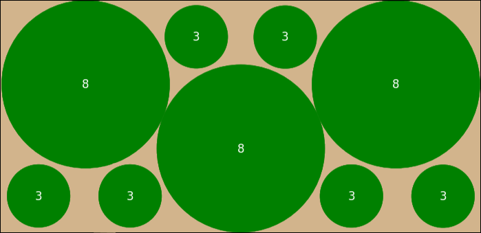
After some trial-and-error, our best manual layout is shown in Figure 4. The layout is symmetrical, with 9 machines of 2 different sizes. The 3 machines consisting of 8 segments each are very close to touching, though not quite. The spaces between the larger machines are not large enough for machines with 4 segments, so we use machines with 3 segments.

This layout irrigates 78.56% of the field's area – a substantial improvement over the 62.10% irrigated by the current installation. More importantly, it has an objective function value of +$251,189 – a substantial $534,147 increase compared with the current installation. Even better, because the NPV of this layout is positive, the investment is worthwhile.

In creating this manual layout, we make two observations that will be important when using a solver to solve the model.

Firstly, larger machines are more profitable. Specifically, the cost of a machine is a linear function of the number of segments. But the yield from a machine is a function of the coverage area, which increases with the square of the number of segments. Therefore, all else being equal, larger machines are better.

Secondly, a machine with only one or two segments makes a loss, while larger machines make a positive contribution to the NPV. For example, a machine comes with one segment as standard, and costs $36,000 to buy and install. An extra segment costs $12,000. Two segments cover an area of 5,027 square metres. The NPV maintenance costs are $7,606 for the pivot and $3,803 for the extra segment. The NPV yield for this machine is $51,614. So, the gross margin (before land purchase and fixed operating costs) is $51,614 - $36,000 - $12,000 - $7,606 - $3,803 = -$7,795. A machine with 3 segments makes a contribution of NPV +$40,919 towards the land purchase and fixed operating costs. Therefore, we need to consider only machines with at least 3 segments (including the built-in segment).

Our manual layout is encouraging, as it tells us that we can certainly do better than simply replicating the current installation. To find out how much better, we need to implement and solve the model.

Implementation

Python code

The model is implemented in Python, using the Pyomo library. The objective function is shown in Figure 5.

Figure 5. Objective function

def objective_rule(model):  # NPV of pivot irrigator investment
    yield_npv = sum(np.pi * (model.segment[m] * SEGMENT_LENGTH)**2 for m in model.Machines) * npv_factor * YIELD_GROSS
    cost_machines = MACHINES * MACHINE_COST
    cost_segments = sum((model.segment[m] - SEGMENTS_BUILTIN) * SEGMENT_COST for m in model.Machines)
    maintain = (MACHINES*MAINTAIN_PIVOT + sum(model.segment[m] - SEGMENTS_BUILTIN for m in model.Machines)*MAINTAIN_SEGMENT) * npv_factor
    operating_npv = OPERATING_COST * npv_factor
    field_cost = FIELD_COST
    return -(yield_npv - cost_machines - cost_segments - maintain - operating_npv - field_cost)
model.obj = pyo.Objective(rule=objective_rule, sense=pyo.minimize)

Solution method

We expect the model to be difficult to solve. But it turns out to be even more difficult than we thought.

First, we tried the open-source Bonmin and Couenne solvers. Both fail to find good solutions in all cases.

Therefore, we modified the model to either call solvers on NEOS Server directly, or manually via a model file. We tried several appropriate commercial solvers including: BARON, Knitro, Filmint, LINDO, and Gurobi. We obtained solutions for trivial cases, but for the more interesting cases with four or more machines, none of these solvers provided useful solutions – even after running for several hours.

Then we tried the MINLP-BB solver (called minlp in Pyomo) via NEOS. Since the model is non-convex, the MINLP-BB solver finds only a locally optimal solution. Importantly, MINLP-BB finds locally optimal solutions in a few seconds. Therefore, we ran it multiple times for each case, with different random initial values for the variables, to increase the likelihood that we find an optimal solution in each case. This is a type of multi-start procedure that is often useful for solving difficult non-linear models. Note that there is no guarantee that we have found an optimal solution in each case. For this model, MINLP-BB is the best solver we tried – by a substantial margin.

Solutions

Best solution found for each case

Figure 6 shows the best solutions we found for the cases with 3 to 14 machines.

The solution for 3 machines is trivial – use the largest machines available. The 3 machines have a gap of 1.5m between them. Although machines with 8 segments are very cost-effective, they don't cover a substantial portion of the field. Their total coverage is 59.62%, even less than the current layout, though at least they are profitable (just).

As we add more machines, the solutions become increasingly complex. The solution for 5 machines foregoes one of the 8 segment machines for a combination of machine sizes that is more profitable. The solutions for 10 or more machines are especially tightly packed, covering more than 80% of the field's area. The most densely packed solution has 12 machines, covering 81.67% of the field's area. The solutions for 13 and 14 machines are slightly less dense, as we need to use smaller machines to pack in the greater number of machines.

Except for the case with 3 machines, we have no guarantee that these solutions are globally optimal. They probably are, though there is a small chance that better solutions exist for some of the cases.

All solutions — Figure 6. Best solutions for each number of machines

Profitability of each case

Figure 7 plots the objective function values for each case, along with the current installation and our manual solution. All the cases have a higher objective function value than the current installation. This illustrates how inefficient the current installation is.

Figure 7. Objective function values for each number of machines

The optimal solution is to have 8 machines, with an NPV of $353,513. This is $636,471 better than the current installation (which, coincidentally, also has 8 machines). Our manual solution is quite good, but its objective function value is $102,324 less than the best solution found by the model, which is more than enough to justify the effort of modelling the situation.

Although cases with more than 8 machines cover a higher proportion of the field, they have increasingly higher initial and maintenance costs, so the extra machines are not worthwhile.

All the cases have alternative optima. That is, at least one machine could change position without changing the objective function value.

Note that, for some cases, it is possible to get higher objective function values by allowing machines with only 1 or 2 segments. But since the machines with 1 or 2 segments make a loss, it doesn't make sense to include them. Removing those loss-making machines leads to solutions with fewer machines that are uniformly worse than the solutions shown in Figure 7.

Chosen solution

Figure 8 shows our chosen solution, which has 8 machines. This layout is the most profitable layout. It is substantially better than the current layout. Most importantly, unlike the current layout, our solution is profitable. Therefore, it is worthwhile proceeding with purchasing the field and installing new pivot irrigators.

Specifically, this layout allows the irrigators to cover 78.56% of the field, which is a significant improvement over the 62.10% for the current layout. The investment NPV of the new layout is +$353,513 compared with -$282,958 for the current layout.

The normal layout for pivot irrigators is a simple grid or perhaps offset rows. Typically, layouts use either a single size of machine, or maybe two sizes at most. Our proposed solution uses five different machine sizes in an irregular layout (though there is a pattern to the layout). For the sake of symmetry, we could position the machine with 3 segments directly south of the machine with 8 segments – there is just enough space to do that.

To summarize, Figure 9 shows a calculation of the total investment value based on our proposed machine layout.

Figure 9. Investment value of proposed layout (NPV)

Relative to the norm, our solution is a radical layout. Our neighbours will certainly be surprised by our new installation. Perhaps they may even be inspired to consider optimizing the layouts of their fields.

Conclusion

In this article we describe a model for optimizing the layout of pivot irrigators in a field – a type of circle packing problem. The model is non-convex, with a non-linear objective function and non-linear constraints, making it difficult to solve to optimality.

The model is built in Python with the Pyomo library. After trying several solvers, including commercial solvers, we found that the MINLP-BB solver is the most suitable for this model. As a result, we're able to design a new pivot irrigation system that substantially improves on the current installation, leading to greater efficiency and improved profitability.

If you would like to know more about this model, or you want help with your own models, then please contact us.

Essential reading

Pivot irrigators in a 100 acre field

We optimally arrange pivot irrigators in a field. This is a type of non-linear circle packing problem, which makes the problem both difficult and interesting.

Pivot irrigators in a 100 acre field