Refactor Python models into modules

26 May 2023

We often need to explore variations of a model. We might need to change model parameters, add/remove constraints, or change the objective function. These variations help us understand how different formulations or parameters affect the optimal solution.

In this article we explore two aspects of working with multiple variations of an optimization model:

• Modularization. We refactor an existing model into modules, consisting of functions located in separate files.
• Adding models. We extend the existing model by adding variations that make efficient use of the modular structure.

Along the way, we look at shallow vs deep copying in Python. This is a topic that often causes subtle bugs, so it is important to understand when working with variations of a model.

Our starting point is an existing model, created by Alireza Soroudi as part of his wonderful Optimization in open-source newsletter on LinkedIn. The specific model is Optimal advisor-advisee matching, used with the kind permission of Dr. Soroudi.

Download the model

The original and refactored files are available on GitHub.

Situation

The situation is described in Dr. Soroudi's newsletter:

Once upon a time in the academic realm, a prestigious university faced a challenge in assigning graduate students to faculty advisors. The students yearned for mentors who could fuel their passion, while the professors sought enthusiastic scholars. Optimization was essential to satisfy both parties and foster harmonious academic journeys.

• The level of preference of Professor i to work with student j is P_i,j.
• The level of preference of Student j to work with Professor i is Q_i,j.

The value of P_i,j (for a given professor i) is different for each student j. This is also true for each student (Q_i,j). As a matter of fact, Professor j has limited capacity for supervising the students.

The question is how to assign all the students to the professors?

We have 50 students and 8 professors. A student's most preferred professor has rank 8, while their least preferred professor has rank 1. Similarly, a professor's most preferred student has rank 50, while their least preferred student has rank 1. A professor's overall satisfaction is the average of their assigned student preferences.

We recommend reading the original article on LinkedIn, to understand how the model works.

Original notebook

Steps in the original notebook

The original notebook has all the code in one file, consisting of the following steps:

1. Import dependencies.
2. Create random data.
3. Plot the data.
4. Define and solve a Pyomo Abstract model.
5. Output and plot the solution.
6. Modify the model and re-solve.
7. Output and plot the solution.
8. Define another Abstract model.
9. Create the Pareto efficient frontier.
10. Plot the Pareto efficient frontier.

Steps 5 and 7 are essentially the same (with minor differences). There are three models, where the second is a variation of the first, and the third duplicates parts of the first.

Optimal solution for the original notebook's second model

Figure 1 shows an optimal solution for the second model:

• Each student wants a score as close to 8 as they can get.
• Each professor wants an average score of close to 50. An average score of exactly 50 is possible if a professor accepts only one student. Otherwise, for example, a professor who has 6 students can achieve a maximum score of (50 + 49 + 48 + 47 + 46 + 45) / 6 = 47.5.

Note that the notebook generates random data, so the solution will differ each time the models are run.

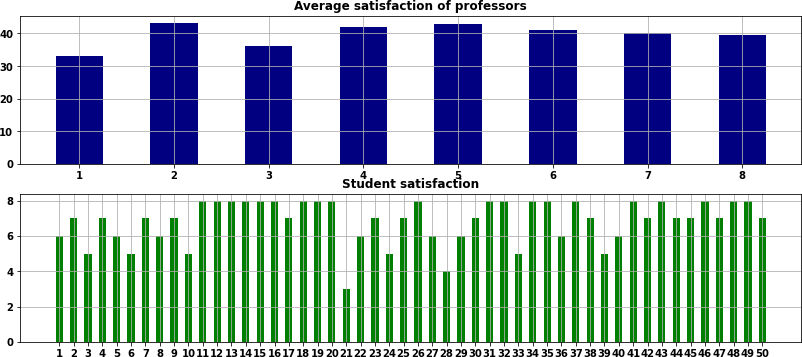
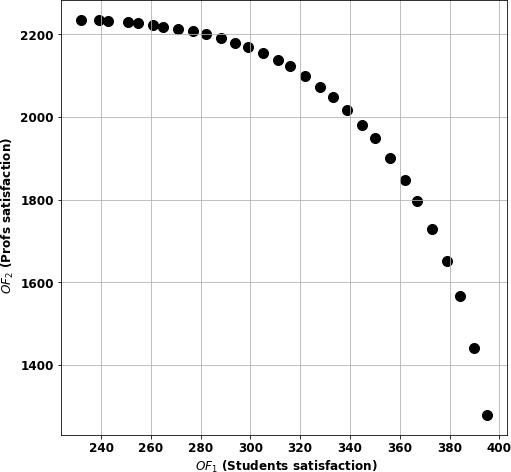
Figure 2 shows the Pareto efficient frontier. That is, given an optimal student satisfaction score, find the optimal solution for the professors.

Evaluation of the original notebook

The original notebook works as expected. The code is short and straightforward to read, so it is easy to understand the models.

But we observe that some students and professors receive relatively low scores. In Figure 1, of the 50 students, 8 receive a score of 5 or less, with the lowest score being 3 out of 8. The professors' scores also vary significantly, ranging from 33.0 to 43.1.

Therefore, we would like to further explore the model behaviour by adding constraints that impose lower bounds on the satisfaction scores, to achieve more equitable scores. There are multiple choices about what the bounds could be, so we'll need multiple variations of the model.

To do that analysis, we could extend the original notebook. But that would make the code significantly longer and more repetitive, making it harder to understand and more difficult to maintain. Instead, we'll refactor the code, dividing it into modules and functions, which will simplify the process of adding more models. This will also allow us to eliminate some code repetition by calling some functions multiple times (e.g., plotting the solutions).

Overview of refactoring

Refactoring approaches

There are two general approaches to refactoring code written by someone else:

• Change only what needs to be changed.
• Comprehensively revise to match your coding style.

We lean towards the former approach, leaving code mostly as is. Therefore, apart from the structural changes needed to modularize the code and add some model variants, we make only a few minor changes to the original code, including:

• Using Concrete rather than Abstract Pyomo models.
• Using Pandas dataframes to output the results in a more compact format.
• Putting spaces around operators, which we prefer for readability.
• Adding adaptable titles to the satisfaction plots.

Objectives for refactoring the notebook

We have two objectives for our refactoring of the original notebook:

• Objective 1: Restructure the code into modules, using functions.
• Objective 2: Add more models, to extend our analysis of the situation.

Objective 1: Restructure the code into modules, using functions

Benefits of modularization

Models are generally easier to understand and maintain when we divide the code into modules. This is especially the case when we have multiple variations of a model.

Each module should have just one, clearly defined purpose. A module may consist of multiple functions, which helps reduce code repetition. We might also want to locate a module's code in a separate file.

Identify key tasks in the original notebook

By examining the original notebook, we identify that it does four types of tasks:

• Data: Create the data used by each of the models.
• Utilities: Calculate satisfaction, create a Pareto frontier, and print results.
• Plots: Display plots of the data and model results.
• Models: Define each of the Pyomo models.

These tasks form the basis for creating modules.

Note that the original notebook generates different random data each time it is run. In our refactoring, we introduce a random seed paramater, random.seed(4), so that the same random data is used each time the models are run. Having a constant data set makes model testing easier.

Use an external file for each module

There are several ways that we could structure the modules. In most of our blog models, we put code into functions, where all functions are in a single Jupyter notebook. For small models, this approach works well. It would work in this situation too.

However, for larger models, having everything in a single notebook becomes unwieldy. Therefore, we illustrate the approach of putting related functions into modules, with each module as a separate Python file. We then read those external files into the Jupyter notebook at runtime:

with open('data.py') as f: exec(f.read())
with open('utilities.py') as f: exec(f.read())
with open('plots.py') as f: exec(f.read())
with open('models.py') as f: exec(f.read())

The Jupyter notebook is our main program, containing only some documentation, setup code, and a cell for each of our models. The process of running a model consists only of calling the functions for each major step, like:

# Model 1: Additive professor and student preferences
model1 = defineModel1()
results1 = opt.solve(model1)
printResult(results1, model1, 'Model 1', '1')

Original and refactored code structures

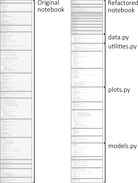
Figure 3 shows an overview of the original code structure (on the left) and the code structure after refactoring (on the right).

The original notebook has 265 lines of code (not counting comments and blank lines) in 15 Jupyter code cells. The refactored notebook has only 47 lines of code in 11 code cells, plus four external Python files that have 230 lines of code in 14 functions, for a total of 277 lines of code. That is, the two versions have about the same number of lines of code – though the refactored version has the bulk of the code in separate files. The refactored notebook also has six models rather than three models.

Note that our first objective is to restructure the code into modules, rather than to reduce the lines of code. In general, although using functions allows us to reduce code repetition, there is some overhead when creating and calling functions in modules, so the code may become longer overall.

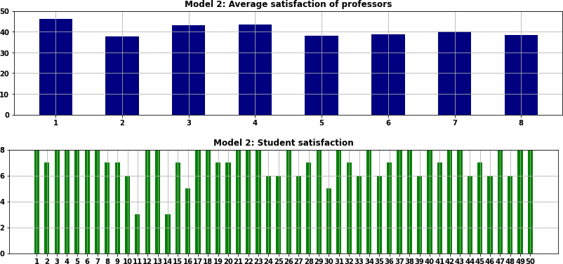
Solution for refactored Model 2

Figure 4 shows the result for our refactored Model 2. Four students receive a satisfaction score of 5 or less, while half the students receive the maximum possible score of 8. The professors receive average satisfaction scores that range from 37.8 to 46.0.

Note that this result differs from the original notebook's second model because that model uses random data which changes each time the model is run. If the original and refactored models use the same random seed, then they produce the same results. This is a characteristic of refactoring – changing the code without changing the behaviour.

Objective 2: Add more models, to extend our analysis of the situation

Lower bound on student and professor scores

We observed that the original notebook's second model produces low satisfaction scores for some people. Our refactored version, Model 2, has the same behaviour.

One way to make the results more equitable is to add constraints that impose minimum scores for students and professors. For the students, this additional constraint ensures that the assigned preference is at least a minimum score:

sum(model.U[i, j] * Q[i, j] for i in model.i) >= model.StudentMinScore

For the professors, the additional constraint is more complex. The satisfaction score for each professor is the average of their assigned preferences. We want to impose a lower bound on the average score, but professors may have different numbers of students. Calculating an average involves dividing by the number of assigned students – but that number is a variable, so dividing would make the model non-linear.

Fortunately, there is a simple way to avoid the non-linearity. Instead of dividing the left-hand-side of the constraint by the professor's number of students, we multiply the right-hand-side by the professor's number of students. The other term on the right-hand-side is the constant minimum score, so all is good. This leads to the constraint for professors:

sum(model.U[i, j] * P[i, j] for j in model.j) >= model.ProfMinScore * sum(model.U[i, j] for j in model.j)

Given a student lower bound assumption we can, through trial-and-error, find the best feasible minimum score for the professors. This is like the Pareto calculation. Of course, adding constraints creates a trade-off: increasing the minimum scores leads to a lower objective function.

We want to explore variations that use three different sets of student minimum score parameters (low, medium, and high values). This requires the creation of three additional models. The models are only slightly different to the models in the original notebook, so we want to copy the existing models and make minor modifications.

Shallow vs deep copy in Python

Before copying the models, let's see how Python handles copying of objects. This is important because we need to understand how copying objects works when we create each of the models.

In some programming languages, when we copy an object, we get a new, entirely distinct object. But Python sometimes doesn't behave like that – for compound objects it creates a new object that shares a reference to the original object. This can lead to unexpected behaviour when working with variations of a model.

To illustrate the issue, we start with two simple objects, \(a\) and \(b\), to which we assign integer values:

Now we assign \(b\) to \(a\), so they both have the same value:

If we change the value of \(a\), then the value of \(b\) remains unchanged:

Similarly, if we change the value of \(b\), then the value of \(a\) remains unchanged:

So far, copying objects has worked as most people expect it to work. But things are different when we copy compound objects.

For example, we create two list objects, \(c\) and \(d\):

Now we assign \(d\) to \(c\), so they have the same values:

If we change an element of list \(c\), then the same element of list \(d\) also changes. This may be surprising behaviour. It happens because \(c\) and \(d\) are no longer separate objects. Instead, they are both pointers to the same object:

Similarly, if we change an element of \(d\), then \(c\) also changes – because they are the same object:

What is happening is that when we assigned \(d\) to \(c\), Python did a "shallow copy" – that is, Python copied only the pointer to the object, rather than copying the object.

To make a separate object, we need to do a "deep copy", which forces Python to make a copy of the object. Deep copying is a function included in the copy library, which we'll use for some of our refactored model variations.

For example, if we create a new list object \(e\):

Then make \(f\), a deep copy of \(e\) so they have the same values:

If we change an element of \(e\), then \(f\) remains unchanged, because they are separate objects:

Similarly, if we change an element of \(f\), then \(e\) remains unchanged:

Sometimes we'll want to do a shallow copy, while at other times we'll want to do a deep copy. It is important that we're clear about which type of copying is required in a specific case.

Model definitions

Returning to the analysis, we want our refactored notebook to include the three models that were in the original notebook plus three variations that explore different lower bounds on the student and professor scores.

That is, we want six models, defined as:

• Model 1. The base model, with additive weights in the objective function. Since the other models are derived from Model 1, only Model 1 has a ConcreteModel() declaration. This model was in the original notebook.
• Model 2. Changes the objective function weights to be multiplicative. This also changes the weights in Model 1 since they point to the same object. This model was in the original notebook.
• Model 3. Adds constraints for lower bounds on the student and professor scores. We do not want Model 1 or Model 2 to include these bounds, so we make the change on a deep copy of Model 2. In terms of the analysis, it would make sense for this model to be positioned after Model 4, but we include it here to illustrate how a deep copy of Model 2 leaves Models 1 and 2 unchanged, so we can use Model 1 as a basis for creating Model 4. This is a new model in the refactored notebook.
• Model 4. Generates an efficient frontier by extending Model 1. Uses a deep copy, so that Model 1 is not changed. Although we created Model 1 with additive weights, Model 2 did a shallow copy so Model 1 now has multiplicative weights. Therefore, Model 4 also has multiplicative weights (though Model 4 doesn't use the weights directly). This model was in the original notebook, except it was created as a new model rather than as a copy.
• Model 5. Explores different values for the student and professor score lower bounds parameters. Does a deep copy of Model 3, so that Model 3 is not changed. This is a new model in the refactored notebook.
• Model 6. Explores another set of different values for the student and professor score lower bounds parameters. This model does not have a function, as we can re-use the function for Model 5 but with different global parameters. This is a new model in the refactored notebook.

All the models are defined in functions. The code within each function is written using a local object called model – ensuring that all model definitions use consistent notation. In the main program, we create objects called model1, model2, etc. When we want a new model to inherit attributes of an existing model, we pass one of these objects to the new model's function. Whether we do a shallow or deep copy of a input model is determined within each model's function.

At each step, we need to be aware of the scope of our object variables. The objects model1, model2, etc. are defined globally, so they are available within any of the functions (after they are created in the main program). However, it would be poor programming practice to change them within the functions, so we use local objects instead.

Sample of model code

Using the model definitions above, we can construct the code for each model.

For example, Model 2 is the same as Model 1, except that we want to modify the objective function weights. Therefore, we create Model 2 by calling its function and passing in Model 1:

model2 = defineModel2(model1)

The function for Model 2 consists only of two lines, plus a line that returns the model with altered weights:

def defineModel2(model):   # Change weights to be multiplicative
    for (i, j) in P:
        model.Coef[i, j] = P[i, j] * Q[i, j]
    return model

Because we return the object that is passed into the function, in effect doing a shallow copy, this function also changes Model 1.

For Model 3, we want to inherit all of Model 2's attributes and add constraints for the minimum student and professor scores. So, we pass in model 2:

model3 = defineModel3(model2)

However, in Model 4 we want to use Model 2 without those additional lower bound constraints. Therefore, when creating Model 3, we do a deep copy so that Model 2 is not changed. This requires separating the passed object, which we call modelInherit, from the model object used in the rest of the function. The first thing we do is make a deepcopy of the inherited model, then we make changes to that new object, independent of Model 2:

def defineModel3(modelInherit):   # Add constraints for minimum professor and student outcomes. Duplicates model, without changing existing model
    model = copy.deepcopy(modelInherit)
    model.ProfMinScore = Param(mutable = True, initialize = ProfMinScore)
    model.StudentMinScore = Param(mutable = True, initialize = StudentMinScore)

    def rule_minForProf(model, i):
        return sum(model.U[i, j] * P[i, j] for j in model.j) >= model.ProfMinScore * sum(model.U[i, j] for j in model.j)
    model.C_Prof_Min = Constraint(model.i, rule = rule_minForProf)

    def rule_minForStudent(model, j):
        return sum(model.U[i, j] * Q[i, j] for i in model.i) >= model.StudentMinScore
    model.C_Student_Min = Constraint(model.j, rule = rule_minForStudent)

    return model

The other models are created in a similar manner, using shallow or deep copying depending on what we want, as defined above.

Results for refactored notebook

Our second objective is to explore the impact of setting a lower bound on the student and professor scores. Having created all the models, we're now able to complete that analysis.

The optimal solution for Model 3, which includes the lower bound constraints, is shown in Figure 5. In Model 3 we set the minimum student satisfaction parameter to be 6. The result is that all students have a satisfaction score of 6, 7, or 8 – significantly better than in Model 2 (where four students received a score of 5 or less, as shown in Figure 4). The professors have a more uniform satisfaction score, though mostly at a lower level than in Model 2.

These results show the trade-off from making the scores more equitable by improving the lowest scores: overall satisfaction is lower. Specifically, the objective function value for Model 2 is 14,326. The objective function for Model 3, which is the same except for the additional lower bound constraints, is 13,544. Therefore, increasing the lowest satisfaction makes the results more equitable, but it has a significant detrimental impact on overall satisfaction.

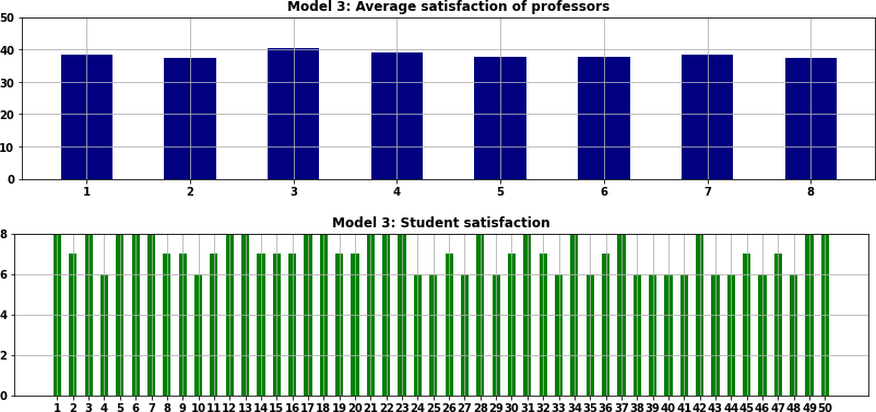
We repeat the analysis in Model 5, with the student's minimum satisfaction set at 5, leading to higher professor satisfaction. Similarly, Model 6 sets the minimum student satisfaction at 7, leading to a much lower average satisfaction for the professors.

Which solution is preferred depends on the importance we place on the satisfaction of the students relative to the professors. By extending the analysis, we have additional information to help us decide which assignment of students to professors is best in our situation.

Conclusion

In this article we refactored an existing Jupyter notebook to make it more modular. The refactoring enabled us to easily extend the original notebook to include additional models, so that we could do more analysis to further explore model behaviour.

For small models, having all the code in a single Jupyter notebook is fine. But as models become larger and more complex, putting all code in a single notebook soon becomes unwieldy. Structuring the code into modules, consisting of multiple functions, can make the code easier to understand and simpler to maintain. Separating much of the code into external files allows us to focus only on a small part of the code at a time, avoiding cognitive overload and reducing the risk of errors in our modelling.

In addition, when working with multiple models, we need to be aware of how Python behaves when doing shallow vs. deep copying. We also need to watch out for scope issues. Both types of issues can lead to unexpected behaviour and bugs if not handled correctly.

If you would like to know more about this model, or you want help with your own models, then please contact us.

References

Soroudi, A. (2023). "Optimal advisor-advisee matching", available at Optimal advisor-advisee matching, published 17 May 2023, accessed 22 May 2023.