Solver Max - Price breaks in a linear programming model

28 April 2023

Price breaks, or volume discounts, are common when buying products in bulk. That is, the marginal cost of additional products falls as volume increases. In a linear program, price breaks are tricky to model because the break points are non-linear discontinuities.

In a spreadsheet, a natural way to model price breaks is to use functions like IF, VLOOKUP, CHOOSE, MIN, and/or MAX. However, those functions are discontinuous, so we can't use the Simplex linear method in Solver. We also can't use the OpenSolver solvers at all when our model includes those functions. We could use Solver's GRG non-linear or Evolutionary methods, but they are not always reliable.

Fortunately, there is a way to express price breaks linearly, by using some binary variables, as described in our article MIP formulations and linearizations.

In this article, we describe an example of how to represent price breaks in a linear programming model, built in Excel using Solver or OpenSolver.

Download the models

The model is available on GitHub

Situation

Figure 1. Incremental prices from each supplier

We own a small cranberry sauce manufacturing business. The recipe is an old, family secret – passed down from generation to generation. Of course, the main ingredient is cranberries.

We use only fresh cranberries. Given our current production, our demand for cranberries is 2,250 kg/week.

There are three local suppliers of fresh cranberries. As shown in Figure 1, two of the suppliers offer a price structure that has incremental price breaks, while the other supplier offers a flat price.

That is:

Premium Fruits. Has an incremental price break structure, starting at $2.00/kg for the first 50 kg, $1.80/kg for the next 50 kg, etc. We have an existing contract to buy 250 kg per week. They can supply up to 2,000 kg per week.
Joe's Cranberries. Sells cranberries with an incremental price break structure, starting at $1.50/kg for the first 100 kg, $1.00/kg for the next 200 kg, etc. They can supply up to 3,000 kg per week.
Bulk Berries. Offers a flat price of $0.75/kg for any quantity. They can supply up to 10,000 kg per week.

Our question is: Which supplier, or combination of suppliers, should we choose to minimize the total cost of our weekly order of cranberries?

Model design

Representing incremental price breaks

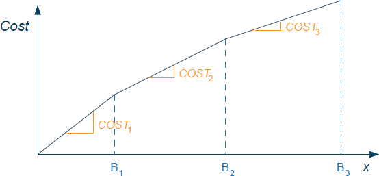
Price break chart — Figure 2. Incremental price break bands

In our article MIP formulations and linearizations we refer to a document from FICO that includes, amongst other things, a linear formulation for representing incremental price breaks.

The structure of the price breaks is expressed in terms of quantity bands, each of which has a price. This structure is shown in Figure 2, which is just another way of showing the pricing structures in Figure 1.

That is, we have incremental price breaks, meaning that the unit cost for items between quantities 0 and $B_1$ (band 1) is $Cost_1$, quantities between $B_1$ and $B_2$ (band 2) cost $Cost_2$ each, etc. This type of incremental pricing structure is exactly the situation we have with two of our cranberry suppliers.

The document also includes a formulation for "all items discounts", meaning that when buying a certain number of items we get discounts on all items that we buy if the quantity is within certain price bands. That formulation is not of interest in this model, but it might be in other situations.

Formulation

The formulation uses binary variables to represent each band of the price function, as shown in Figure 3. Note that we have generalized the document's formulation to have any number of price bands.

Figure 3. Incremental price break formulation

\begin{alignat}{1} &\text{Constraints} \\ & \quad \text{Total purchase} &= & \quad \sum_{i=1}^n x_{i} \tag{1}\\ & \quad (\text{B}_i - \text{B}_{i-1}) \times b_{i+1} \quad &\le & \quad x_i \tag{2} &\begin{array}{l} \forall \ i \in \{1 \ldots n-1\} \\ \end{array} \\ & \quad (\text{B}_i - \text{B}_{i-1}) \times b_{i} &\ge & \quad x_i \tag{3} &\begin{array}{l} \forall \ i \in \{1 \ldots n-1\} \\ \end{array} \\ & \quad (\text{B}_n - \text{B}_{n-1}) \times b_{n} &\ge & \quad x_n \tag{4} \\ & \quad b_i &\ge & \quad b_{i+1} \tag{5} &\begin{array}{l} \forall \ i \in \{2 \ldots n\} \\ \end{array} \\ \\ &\text{Variables} \\ & \quad b_{i} \quad && \quad \text{Binary, use band } i &&& \quad \tag{6} \\ & \quad x_{i} \quad && \quad \text{Purchase quantity in each band } i &&& \quad \tag{7} \\ \\ &\text{Data} \\ & \quad \text{B}_{i} \quad && \quad \text{Breakpoint quantity for band } i &&& \quad \tag{8} \end{alignat}

Note that Equation (4) is a special case for the last band. With careful construction of the formulae, we can collapse this constraint into Equation (3).

The rest of our model formulation is straightforward – it simply repeats the price band structure for each supplier and ensures that we meet demand at minimum cost. We also require that the existing contract quantity with Premium Fruits is fulfilled.

Implementation

Price bands data

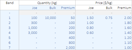
To implement the model in Excel, we start with the data, as shown in Figure 4.

For each supplier, we list the quantity break points for each band, along with the price for all quantity within that band. We've allowed up to 7 bands, though this could easily be extended.

The Bulk Berries supplier doesn't offer price breaks – they have a flat price for all quantities. This structure can be accommodated within our model by specifying their data to have just one band.

Equation (5) of the formulation starts with the second band, because it refers to the previous band. We can simplify construction of the model by introducing an empty dummy band zero, to avoid this special case. This dummy band has hard-coded quantities and prices all equal to zero.

Note that the suppliers can have different quantity break points and different numbers of bands. The model handles those differences automatically.

Variables we'll need

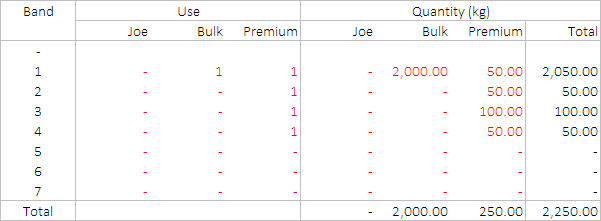
Price band selection variables — Figure 5. Price band use and quantity variables

We need two sets of variables, as shown in Figure 5:

Use. A binary variable to indicate whether we're using each band. These variables correspond to $b_i$ in the formulation, though we have an additional dimension to represent each supplier.
Quantity (kg). The quantity of cranberries purchased within each price band. These variables correspond to $x_i$ in the formulation, though we have an additional dimension to represent each supplier.

Note that both Solver and OpenSolver may set some of the Use binary variables to 1, even when that band is not used. This occurs because our model has no penalty for setting those variables to a non-zero value, provided the quantity variables are zero. That is, this quirk does no harm. We could tidy up the model by forcing the stray Use variables to zero by giving them a very small penalty in the objective function, though it isn't necessary to do so.

Constraints to create price breaks

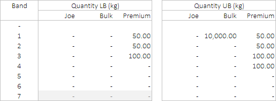
Figure 6 shows the two sets of constraints that represent:

Equation (2): the lower bounds on the band quantities.
Equations (3) and (4): the upper bounds on the band quantities.

In the spreadsheet, these two constraints are a direct translation of the formulation, simplified to consolidate the special cases.

We also have constraints that represent Equation (5), applied directly to the Use variables in Figure 5. Those constraints ensure that if we use a band, then we must also use all lower quantity bands. This is necessary because the prices decline as quantity increases. Therefore, the solver would prefer to use higher quantity bands first – because they are cheaper. But such a solution isn't allowed, so we need to forbid it.

Solver model

Objective function

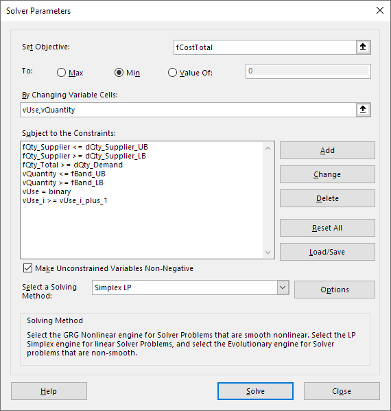
The Solver model is shown in Figure 7. Our objective is to minimize the total cost of buying the required demand for cranberries.

Variables

The model has two sets of variables:

vUse. Binary variable indicating whether to use each price band for each supplier.
vQuantity. Purchase quantity in each price band for each supplier.

Constraints

The constraints are:

fQty_Supplier >= dQty_Supplier_LB. Total quantity for each supplier must be at least the minimum quantity for that supplier. We use this to implement the existing contract with Premium Fruits.
fQty_Supplier <= dQty_Supplier_UB. Total quantity for each supplier must be no more than the maximum quantity available from that supplier.
fQty_Total >= dQty_Demand. Overall total quantity must be at least the required demand. Since we're minimizing cost, the model will exceed demand only if it must (i.e., if the minimum quantities from the suppliers sum to more than the demand).
vQuantity <= fBand_UB. The quantity in each band from each supplier must comply with Equation (2).
vQuantity >= fBand_LB. The quantity in each band from each supplier must comply with Equations (3) and (4).
vUse_i >= vUse_i_plus_1. Requires that lower band are used first, as specified in Equation (5).

Solution method

All the model's relationships are linear, along with some binary variables, so we can use the Simplex method. This model is sufficiently small that either Solver or OpenSolver can be used.

Analysis

Base Case

The optimal solution for our Base Case (also known as Scenario A) is shown in Figure 8.

Results for Scenario A — Figure 8. Results for Base Case, Scenario A

We purchase the contracted 250 kg from Premium Fruits, but nothing more. The remainder of our demand is met by Bulk Berries, with a quantity of 2,000 kg. The total cost is $1,920.00.

The average cost for Premium Fruits is very high, at $1.680/kg, compared with the cost of $0.750/kg for our purchase from Bulk Berries – so it is easy to see why we limit our purchase from Premium Fruits to only the contracted quantity.

But why didn't we purchase anything from Joe's Cranberries? Given Joe's price breaks, the cost of 2,000 kg would be $1,510 ($10 more than from Bulk Berries). The average price would be $0.755 – slightly more expensive than the $0.750/kg for Bulk Berries. Therefore, the optimal solution is to not buy any quantity from Joe's Cranberries.

Additional scenarios

To explore how the optimal solution changes if we alter the demand, we consider some additional scenarios. That is, we vary the demand to see how that affects which suppliers to choose, given our other constraints. We also see how our choice of supplier(s) changes once the existing contract with Premium Fruits ends.

Detailed results are shown in Figures 9 and 10.

Figure 9. Scenario results: Quantities and costs

Figure 10. Scenario results: Average prices

In summary:

1. Base Case. We are required to buy at least 250 kg from Premium Fruits. The remainder of the demand is purchased from Bulk Berries, at a price of $0.75/kg, as they are cheaper than Premium Fruits and Joe's Cranberries.
2. Increase demand to 2,500 kg. Increasing demand reduces the average cost for Joe's Cranberries to $0.738, which is less than the $0.75/kg cost for Bulk Berries. Therefore, we switch to buying from Joe (apart from the contracted quantity from Premium Fruits).
3. Increase demand to 3,500 kg. If the demand increases further, then Joe's Cranberries cannot supply our demand (because they have a capacity of 2,000 kg/week), so we buy from all three suppliers.
4. After Premium contract ends. After the Premium Fruits contract ends, Joe is the cheapest supplier for our current demand quantity. Premium Fruits is always more expensive than the other suppliers, so without the contract we would not choose to buy from Premium Fruits.
5. After Premium, demand 2,500 kg. Joe remains the cheapest supplier if demand increases slightly after the Premium Fruits contract ends.
6. After Premium, demand 3,500 kg. Like Scenario 3, if demand increases further, then Joe cannot meet all our demand. Therefore, we need to buy from both Joe and Bulk Berries – though not from Premium Fruits, who are too expensive.
7. After Premium, demand 2,067 kg. The crossover point between Joe and Bulk Berries occurs where the average cost for Joe equals the cost for Bulk Berries – i.e., at $0.75/kg. When the demand is 2,067 kg, the average price for Joe is $0.74998/kg, so Joe is very slightly cheaper than Bulk Berries. For demand more than 2,067 kg, Joe's marginal cost is $0.60/kg, which is less than the $0.75/kg for Bulk Berries, so we would buy from Joe.
8. After Premium, demand 2,066 kg. But if demand is 1 kg less, then the average price for Joe is $0.75005/kg, so Bulk Berries is very slightly cheaper than Joe. Therefore, if demand is 2,066 kg or less, we would switch to buying all the demand from Bulk Berries.

Conclusion

In this article we've describe how to solve a linear programming model that includes incremental price breaks from multiple suppliers. The model formulation applies a linearization technique that uses binary variables to represent each of the price bands.

The model is built in Excel, though the same technique could easily be applied to a model built using other tools, such as Python.

We also solved several scenarios, to explore how the price breaks behave under a variety of assumptions. The key factor in determining which supplier to choose is the average cost over the allocated volume.

If you would like to know more about this model, or you want help with your own models, then please contact us.

References

FICO Xpress Optimization (2017). "MIP formulations and linearizations: Quick reference", PDF available from MIP formulations and linearizations. Online version also available at FICO Xpress optimization help.

Price breaks in a linear programming model