Crossword MILP - Model 2

10 January 2024

In Part 1 of this series, we formulated a Mixed Integer Linear Program (MILP) for compiling crossword puzzles. Model 1 works OK, provided the crossword grid is small, not too dense, and the lexicon isn't too large. But as the grid gets denser and/or the lexicon gets larger, Model 1 struggles to find solutions.

We can do better. Model 1 uses a general formulation, where we specify the form of each constraint and then let the solver work out which variables and constraint instances aren't needed, given a specific data set. For many models, this approach is sufficient – largely because modern optimization solvers are very good at eliminating unnecessary terms in a model, especially in the presolve phase.

But solvers use general-purpose procedures for tightening models. Sometimes we can make use of our knowledge about the specific situation to help the solver.

In this article, we discuss techniques for fine-tuning the model-building process in Pyomo, to make a smaller and faster model. Specifically, we:

• Select only those words in the lexicon that fit in the current grid.
• Pre-populate some grid word slots with random words, to give the solver a head start.
• Omit constraint terms that don't meet some criteria.
• Skip some constraint instances entirely.
• Fix some binary variable values at zero, when we know they cannot have a value of one.

These steps tighten the model, making it easier for the solver to find a solution. We'll then look to solve larger crossword compilation problems.

Download the models

The models described in this series of articles are built in Python using the Pyomo library.

The files are available on GitHub.

Situation

We want to create a model that compiles crossword puzzles. That is, given a grid design and a word lexicon, find a set of words that fit in the grid while complying with the crossword's rules.

Details of this situation are presented in Part 1 of this series.

Model 2 design

Tightening the model

We usually leave the solver's presolve process to tighten the model by eliminating variables and constraints that are not needed, and to reformulate the model in other ways that make it easier/faster to solve. The automated presolve process is sufficient for most models. But our crossword compilation model is difficult to solve – especially when using a large, dense grid and extensive lexicon. Therefore, we need to help the solver to tighten the model.

Restrict the lexicon to words that fit the grid

Both Models 1 and 2 have a feature in which we select a random sample of words from the lexicon. We do this to constrain the size of model.

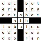
In choosing the words, Model 1 simply selects the specified number of candidate words from the lexicon. For example, the Gutenberg lexicon contains 35,259 words of length 2 to 15 characters. However, grid 7-2, as shown in Figure 1, has words of lengths 3 and 7 characters only. In the Gutenberg lexicon there are 1,224 words of length 3 and 5,350 words of length 7, so we can use only 6,574 of the 35,259 words, i.e., we can eliminate up to 81% of the words when constructing the model for grid 7-2, depending on the sample size we specify.

Restricting the sample words to only those word lengths that appear in the grid has two effects:

• The model may be smaller. A smaller size model is usually faster to solve.
• When using a sample of the lexicon, there are more candidate words that fit the grid. Having more words makes it more likely that a sample of words will produce a feasible solution.

The lexicon filtering, to include only words that fit in the grid, is done in Model 2's data preparation process. The specific code is shown in Figure 2. The random sample is taken from the filtered list.

SelectedWords = []   # Select words as candidates only if they match the grid's word lengths
GridWordLengths = []   # Length of words in the grid
for g in Model.GridLengths:
    if pyo.value(Model.GridLengths[g]) not in GridWordLengths:
        GridWordLengths.append(pyo.value(Model.GridLengths[g]))
GridWordLengths.sort()   # e.g. [4,5,9,15]
for c in range(0, len(Word)):
    if len(Word['Candidate'][c]) in GridWordLengths:
        SelectedWords.append(c)   # Subset of lexicon words, included only if they fit in the grid

Populate some grid words slots with random words

A key issue with Model 1 is that there are potentially thousands of words that will fit in each grid word position. If we pre-populate a few of the grid word positions with randomly selected words that fit, then the solution space is considerably reduced.

However, we need to be careful not to pre-populate too many words, as that increases the risk of making the puzzle infeasible. Similarly, we should avoid pre-populating the grid with words that crossover, as they will almost certainly be infeasible.

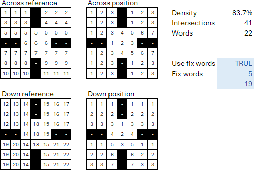
In the grid definition Excel file, we include a named range that lists grid positions that are to be pre-populated with words randomly selected from the lexicon. There is also a switch that turns this feature on/off for the current grid. For example, the grid definition for 7-2 is shown in Figure 3. We specify that grid word positions 5 (across) and 19 (down) are to be pre-populated. We've carefully picked two word positions that don't intersect in this grid.

In the model building process, we fix at a value of 1 the binary allocation variable for each pre-selected candidate word and grid position. This is done using Pyomo's .fix(1) function, appended to a specific variable. For more about fixing variable values, see the Pyomo documentation Fixing variables and re-solving (though we're fixing the values before solving the model, rather than re-solving).

A similar process could be used to pre-populate grid positions with specific words, rather than random words – though we haven't implemented that feature.

Omit constraint terms

In addition to filtering the lexicon to include only words that fit somewhere in the grid, we filter the terms of each constraint and the objective function such that only words that fit a specific grid position are considered.

For example, in Model 1, for each grid position, we sum the allocation variables for all candidates. That is, Model 1's Model.EachPositionOnce constraint is shown in Figure 4.

def rule_PosOnce(Model, g):   # Allocate exactly one candidate to each grid word position
    return sum(Model.Allocation[c, g] for c in Model.Candidate) == 1
Model.EachPositionOnce = pyo.Constraint(Model.GridWords, rule = rule_PosOnce)

But most words won't fit in a specific grid position, so most of the constraint terms are unnecessary. We could rely on the solver to identify and eliminate these unnecessary terms, either during the presolve phase or while solving – though it may not do so entirely.

It is better if we eliminate those terms ourselves, using our knowledge of the situation's specific structure. For example, Model 2's Model.EachPositionOnce constraint includes a test to include only the variables where the candidate word length and the grid word length are equal, as shown in Figure 5. We manually construct a summation of just those terms.

def rule_PosOnce(Model, g):   # Allocate exactly one candidate to each grid word position
    ColumnTotal = 0
    TermsAdded = 0
    for c in Model.Candidate:
        if pyo.value(Model.Length[c]) == pyo.value(Model.GridLengths[g]):   # Candidate word length must match grid word length
            ColumnTotal += Model.Allocation[c, g]
            TermsAdded += 1
    if TermsAdded == 0:
        return pyo.Constraint.Skip
    else:
        return ColumnTotal == 1
Model.EachPositionOnce = pyo.Constraint(Model.GridWords, rule = rule_PosOnce)

We apply similar filtering to the other constraints, and in the objective function. This filtering significantly increases the model's code complexity – we'll soon test to see if it is worth it.

Skip some constraint instances

It is possible that our filtering might omit all terms in a constraint. Such an empty constraint will produce a Pyomo error.

To avoid that error, we skip each instance of a constraint that is empty. We do that in Figure 5 above by counting the number of terms added and, if that is zero, returning the Pyomo command pyo.Constraint.Skip. In that case, the current instance of that constraint will not appear in the model.

Fix some binary variable values at zero

In addition to only including variables where the candidate word length equals a grid word position's length, we also do the opposite. That is, we fix at zero all allocation variables where a candidate word length doesn't match a grid word length, as shown in Figure 6.

# Fix some variables. Replaces the rule_Fit constraint. This constraint substantially reduces solve time
for g in Model.GridWords:   # Reduce variables by fixing allocation variables to zero if candidate word length doesn't match grid word length
    for c in Model.Candidate:    
        if pyo.value(Model.Length[c]) != pyo.value(Model.GridLengths[g]):
            Model.Allocation[c, g].fix(0)

This fixing of variables is done outside the constraints. For most grids, this substantially reduces the number of variables the model needs to consider, which sometimes reduces the solve time substantially.

Performance of Model 2 compared with Model 1

To illustrate the impact of the model tightening steps outlined above, let's compare Model 1 and Model 2 for the 7x7 grid 7-2 (shown in Figures 1 and 2). We introduce the tightening steps incrementally.

Effect of restricting the lexicon to words that fit the grid

Restricting the lexicon to only those words that fit in a specific grid has a significant effect on the performance of the model.

If we don't specify a smaller sample, then Model 1 uses all 35,259 words in the Gutenberg lexicon, irrespective of the grid's word lengths. Initially, for grid 7-2, Model 1 has 775,698 binary variables and 5,096,746 non-zeros. Gurobi's presolve reduces the model to 105,714 binary variables and 821,002 non-zeros. That is, presolve eliminates more than 80% of the variables and non-zeros before it starts the solve process. Gurobi takes 774 seconds to find a feasible solution. The overall run time, including data preparation, model building, and output is 967 seconds.

Model 2 uses only 6,574 words from the lexicon, after filtering out all words other than those of length 3 and 7 characters. Initially, Model 2 has 144,628 binary variables and 953,368 non-zeros. Presolve reduces the model to 43,432 binary variables and 282,232 non-zeros. Gurobi takes 782 seconds to find a feasible solution. The total run time is 821 seconds.

For both models, the presolve process does most of the work. But our model tightening helps too, reducing the model size by 59% for the variables and 66% for the non-zeros after presolve. Even though Model 2 is smaller, the solve times of the two models are almost the same. The benefit of trimming the lexicon is that it takes less time to build the model, with the total run time being reduced by 15%.

Pre-populating some grid words

When we pre-populate a few grid positions with randomly selected words from the lexicon, we substantially reduce the size of the solution space.

With this feature added, Model 2 initially has 144,628 binary variables and 953,352 non-zeros (almost identical to the previous step). Presolve reduces the model by more than two-thirds compared with the previous step, to 14,431 binary variables and 72,056 non-zeros.

Gurobi takes just 9 seconds to find a feasible solution – a large reduction. The overall run time is 48 seconds, so most of the run time is preparing the data, building the model, and writing the output. No doubt we could improve the efficiency of our data handling, model building, and output code, but that isn't something that we have focussed on.

Additional model tightening steps

Adding the other model tightening steps, omitting terms and fixing variable values, further reduces the initial model size and solution time.

After including the additional features, Model 2 initially has 144,628 binary variables (same as the previous step) and 302,746 non-zeros (68% reduction compared with the previous step). Presolve reduces the model to 14,689 binary variables and 73,159 non-zeros (slightly more than the previous step). Gurobi takes 8 seconds to find a feasible solution. The overall run time is 41 seconds.

For grid 7-2, these additional tightening steps reduce the times by only a small amount. For some larger models, they have more impact.

Overall effect of the model tightening steps

The effects of our model tightening efforts are summarized in Figure 7.

Overall, after presolve, our model tightening reduces the number of variables for grid 7-2 by 86%, the solve time (in seconds) by 99%, and the total run time by 96%. The trade-off is that the code for Model 2 is substantially more complex than Model 1, even though the formulation is essentially the same. But that trade-off seems worthwhile, given the large improvement in performance for Model 2 compared with Model 1.

Solving more complex and larger grids

Model 2 performs much better than Model 1. So, we can now try solving some larger and/or more complex grids using Model 2.

In the previous article, we looked at single and double word squares. The tightening steps described above are of little or no benefit for that type of puzzle. That is, word squares are 100% dense, so there are few, if any, terms that our steps can eliminate. Worse, pre-populating a word square with even one randomly selected word almost certainly makes it infeasible. Model 2, like Model 1, is not well-suited to solving word squares.

So, for the remainder of this article, we focus on traditional crossword grids.

7x7 grid

In the previous article, we were able to solve low and moderate density 7x7 grids, specifically grids 7-1 and 7-2, but we failed to solve the much denser 7-3 grid using Model 1.

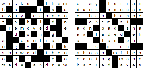
Model 2 performs much better, finding many solutions for grid 7-3 – typically taking one to a few minutes per solution (using the full Gutenberg lexicon). Some of the solutions are shown in Figure 8. Finding these solutions demonstrates how much better Model 2 is compared with Model 1.

11x11 grid

It is time to ramp up the size and/or complexity of the crossword grids we're solving.

An 11x11 grid is a popular crossword size – large enough to provide a challenge, but without containing many words. Figure 9 shows two 11x11 crossword grids:

• The grid on the left is a British-style crossword. It has 20 words, 24 crossovers, and density of 69%. Using the full Gutenberg lexicon (of which 13,550 words fit this grid), it typically takes a few seconds to solve (first feasible solution).
• On the right is a denser American-style crossword. It has 52 words, 97 crossovers, and density of 82%. This more difficult puzzle typically takes about 10 minutes to solve – though it is much more likely to be infeasible, given a specific random sample of the lexicon.

15x15 grid

Figure 10 shows three 15x15 crossword grids:

• The grid on the left is a British-style crossword. It has 29 words, 60 crossovers, and density of 72%. Using the full Gutenberg lexicon, it typically takes about 20 seconds to find a feasible solution.
• In the middle is a simple American-style crossword. It has 82 words, 113 crossovers, and density of 73%. It is difficult to find solutions using the Gutenberg lexicon, as it simply doesn't contain enough words. Most solutions were found using a sample of 20,000 words from the Large lexicon. Even with 20,000 words, this grid is likely to be infeasible, so we needed many model runs to obtain the solutions we found. When a solution is found, it typically takes 5 to 10 minutes to solve – though some random word samples failed to find a solution at our limit of 1 hour run time.
• On the right is a more typical American-style puzzle. It has 78 words, 189 crossovers, and density of 84%. We were unable to find a solution for this difficult puzzle, even with large sample sizes and running the model for 12+ hours.

The issue with the 15x15 puzzle on the right is that it is very dense and has many word crossovers. These two grid features make a puzzle very difficult to compile – both for humans and for our optimization model.

21x21 grid

Figure 11 shows a 21x21 crossword grid. It has 92 words, 148 crossovers, and moderate density of 70%. Using a sample of 20,000 words from the Large lexicon, the solve time is typically around 1 to 3 minutes to find a feasible solution – of which we found several.

However, most random seeds produce infeasible problems, even with a large random sample of the lexicon, so the overall run time required to find solutions is much longer. Processing the data and building the model is quite time consuming, taking around 4 minutes per run (i.e., usually more than the solve time).

29x29 grid

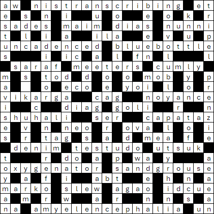
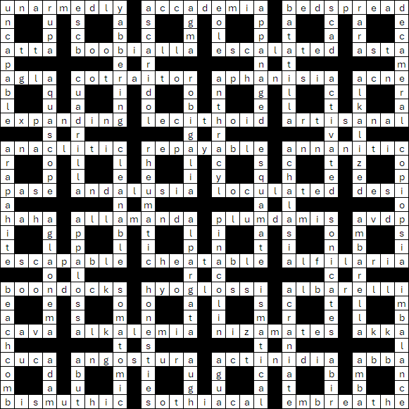
Figures 12 and 13 show two 29x29 crossword grids:

• Grid 29-1, in Figure 12, has 84 words, 144 crossovers, and low density of 59%. Using a sample of 10,000 words from the Large lexicon, solutions are rare – almost all random word samples are infeasible. Increasing the sample size to 20,000 words yields more solutions, which solution times of between a few minutes and 30 minutes (when feasible).
• Grid 29-2, in Figure 13, has 92 words, 148 crossovers, and density of 70%. Using a sample of 20,000 words from the Large lexicon, each solution takes around 30 to 45 minutes to find, though most random seeds produce infeasible problems. A larger sample of the lexicon increases the chances of a run being feasible, but it also usually increases the run time.

Although grid 29-2 is only moderately more complex than grid 29-1, 29-2 is much harder to solve. This is, in part, due to grid 29-2 having a more diverse range of word lengths. Grid 29-1 has only two word lengths (4 and 9 characters), while grid 29-2 has several word lengths. For a sample of a specific size, more word lengths means fewer words of each length for the solver to choose from.

Alternative objective functions

Our focus has been on feasibility, rather than optimality, so we usually stop the solver when it finds a first feasible solution. Even so, the form of the objective function might matter.

A limitation of the objective function we've been using is that it offers the solver little traction for finding a solution. Our objective is a weighted average frequency of either word usage (Gutenberg lexicon) or character occurence (Large lexicon). The issue is that the frequency provides essentially no guidance to the solver in terms of finding a solution. It might be that the solver spends a lot of time trying to improve the weighted average frequency of allocated words, when that value tells the solver little or nothing about how to comply with the constraints.

So, we have added a couple of alternative objective functions to Model 2, to see if they help the solver. The objective function can be chosen using the ObjectiveChoice option in the model:

• Option 1, Allocated words weighted by frequency. This objective was used in Model 1 and throughout the analysis so far for Model 2.
• Option 2, Allocated words. A simple sum of the candidate allocation binary variables. At a feasible solution, the objective value will be the number of grid word positions. This is very similar to the objective that Wilson used in his 1989 paper.
• Option 3. Number of intersections with the same letter. We have a constraint that requires the crossover cells of words to have the same letter – this seems to be the most difficult constraint to comply with. This objective looks to maximize the count of those cells. The idea is that, perhaps, counting the crossovers with matching letters might help the solver meet the crossover constraint. At a feasible solution, the objective value will be the number of crossover cells.

For some grids, Options 2 and 3 perform much better than Option 1. For example, with grid 7-2, using the whole Gutenberg lexicon and random seed of 1, Option 1 finds a feasible solution in 8.1 seconds (solver time only). Option 2 is faster, finding a feasible solution in 3.2 seconds. Option 3 is even faster, taking 2.2 seconds to find a first feasible solution. So, the alternative objective functions do help in this case, reducing the solve time by 73% for Option 3 compared with Option 1.

But as the grids get larger, the benefit of the alternative objective functions seems to diminish. For grid 15-1, Options 2 and 3 each reduce the time to first feasible solution by around 25% – which is useful, but not large. In the case of Option 3, building the objective function requires additional processing time, which erodes the benefit it provides.

For Options 2 and 3, the solver identifies almost immediately what the optimal objective function value will be (unlike for Option 1, where the optimal value is not so obvious). Unfortunately, at least for the more difficult cases, knowing the optimal objective function value is only somewhat useful in helping the solver find a feasible solution.

Perhaps a better objective function would further improve the performance of Model 2? We're open to ideas.

A final puzzle

We've achieved our goal of compiling crossword puzzles of realistic size with a large lexicon.

Model 2 is capable of solving large grids, provided they have moderate density and a moderate number of crossovers. But large American-style crossword grids, with high density and many crossovers, are beyond the model's capability to solve in a reasonable time.

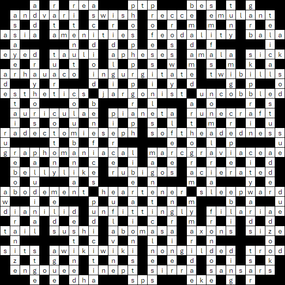
Like many crossword enthusiasts, we've spent far too long working on our crosswords. So, a final crossword is shown in Figure 14.

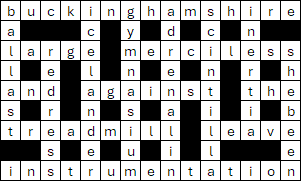
This puzzle has many crossovers, including several areas that are, or are like, word squares. Consequently, this is quite a difficult puzzle to solve. Using a sample of 50,000 words from the Large lexicon, this grid typically takes 1 to 1.5 hours of solve time per feasible solution (using objective Option 3), plus a substantial model-building time. It seems like a fitting way to end our exploration of using a MILP to compile crossword puzzles.

Conclusion

This article concludes our attempt to use a Mixed Integer Linear Program (MILP) for compiling crossword puzzles.

Model 1 works well for compiling small, relatively simple traditional crossword puzzles using a lexicon of up to a few thousand words. Model 2 refines Model 1 by using some advanced techniques to tighten the model. Model 2 works well for larger and more complex crossword puzzles. It can also handle a lexicon with tens of thousands of words. Both models struggle to compile medium-sized single and double word squares, though that style of crossword isn't our focus.

The open-source HiGHS solver can solve some of our examples in a reasonable time. However, the larger and/or more difficult examples need the power of the commercial Gurobi solver to find feasible solutions in a reasonable time.

As our example puzzles get larger and more complex, we have approached the limits of what our model can do. That isn't surprising, as a MILP is not an ideal tool for compiling crosswords – there exist specialized search tools that are better suited to the task.

Nonetheless, we've achieved our goal of using a Mixed Integer Linear Program to compile crossword puzzles of realistic size with a large lexicon. We've also illustrated some techniques that you might find useful in working with your models.

If you would like to know more about this model, or you want help with your own models, then please contact us.