Julia/JuMP vs Python/Pyomo

22 June 2023

In this article we develop an optimization model in the Julia programming language, using the JuMP mathematical optimization package.

The focus is on introducing Julia/JuMP, by replicating the Production Mix model that formed the basis of our article series looking at several Python optimization libraries.

Our objectives are to:

• Write a linear programming model using Julia/JuMP.
• Compare the model with an equivalent model written using Python/Pyomo.

Although Julia/JuMP is not yet widely used outside universities, we expect that it will become an important tool for optimization modelling over the next few years.

Download the model

The model is available on GitHub.

Introducing Julia/JuMP

Julia and JuMP are recent innovations

Julia is a relatively new programming language, first released in 2012, with version 1.0 released in 2018. Julia is designed for numerical analysis and scientific computing applications.

JuMP is a Julia package for representing and solving mathematical optimization problems. Version 1.0 of JuMP was released in 2022, though its origins date back to 2013. JuMP currently has access to more than 30 solvers, covering a wide range of model types.

Julia has a small user base compared with Python. But Julia is increasingly being taught in universities, especially for data science and related applications. Therefore, as those students move into the work environment, we expect that Julia will become more widely used outside of academia in the next few years.

Set up Julia/JuMP for use in Jupyter Lab

Setting up Julia and JuMP is straightforward. The steps we took, using Windows PowerShell on our Windows 10 system, are outlined below. Your mileage may vary.

Set up steps:

• From a PowerShell command prompt, install Julia: winget install julia -s msstore
• Check that Julia installed correctly, by running julia at the command prompt. In our case, we installed Julia version 1.9.0.
• From the Julia command prompt, add Julia to Jupyter Lab (which was already installed), by running: using Pkg; Pkg.add("IJulia")
• Install JuMP: Pkg.add("JuMP")
• Install CBC solver: Pkg.add("Cbc")
• Install other solvers, one at a time, using Pkg.add with the exact names: GLPK, HiGHS, Ipopt, Couenne_jll (includes Bonmin_jll), NLopt, and NEOSServer
• Install some packages that we'll use, including Printf, DataFrames, PrettyTables, and JSON
• You can get a list of installed packages using Pkg.status()

Then open Jupyter Lab, which now has an option to create notebooks using Julia, in addition to Python (which we had installed earlier).

Situation

The Production mix situation is a typical small linear programming problem. That is, the situation we're modelling is:

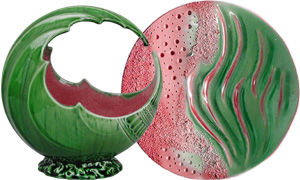
• You own a boutique pottery business, making two types of large ornamental pieces: Lunar Orbs and Solar Discs (known succinctly as Discs and Orbs), as shown in Figure 1.
• Your objective is to maximize gross profit margin per week.
• You need to decide the number of units of Orbs and Discs to produce each week.
• Production is constrained by staff hours, availability of materials, and experience about the number of units of each product that you can sell.

The sales experience constraint means that production of Orbs must be less than or equal to twice the production of Discs.

Model formulation

The linear programming model formulation is identical to the formulation we used in the Production Mix series of articles. The specific formulation is shown in Figure 2.

Implementing the model in Julia/JuMP

Program structure

Our Julia program structure is like our typical Python program structure. This model is small, so we have the whole program in a single Jupyter notebook, though the data is in an external JSON file.

The notebook consists of the following modules:

• Libraries. We import several libraries, including: JuMP, HiGHS, DataFrames, and JSON.
• Globals. A key difference between Pyomo and JuMP is that a Pyomo model object can include all the model's parameters and sets. A JuMP model object doesn't have the capability. Instead, we create a Julia structure struct data type to store and pass our data around the model. A struct must be declared to have global scope.
• Data. We read the model's data from an external JSON file, storing each item in the structure declared above. A structure is highly versatile, being able to store many different data types. We store simple data types, like strings, reals, and integers, along with complex data types like vectors and dictionaries.
• Model. Defining a model in JuMP is like defining a model in Pyomo, using notation that reflects the way a mathematical formulation is typically presented. We can also choose a different solver and set solver options.
• Reporting. We print details of the solution, including sensitivity analyses for the variables and constraints.
• Main. In the main program, we read the data, define the model and options, solve the model, and output some reporting.

Defining the model in JuMP is straightforward

JuMP provides specific objects for variables, constraints, and the objective function. In this example, our model is defined in a function, as shown in Figure 3.

We have a variable for the production of each product, three constraints, and an objective of maximizing the margin we make from selling the products.

function definemodel(data)   # Define the model
    model = Model()
    @variable(model, data.varlbounds <= production[p in data.products] <= data.varubounds)
    @constraint(model, cpeople, sum(data.people[p] * production[p] for p in data.products) <= data.hours)
    @constraint(model, cmaterials, sum(data.materials[p] * production[p] for p in data.products) <= data.kg)
    @constraint(model, csales, sum(data.sales[p] * production[p] for p in data.products) <= data.saleslimit)
    @objective(model, Max, sum(data.margin[p] * production[p] for p in data.products))
    return model
end;

Note that, unlike most Julia/JuMP examples we've seen, our model uses indexed objects. For example, most examples would write the cpeople constraint like:

@constraint(model, cpeople, 12.5Disc + 10.0Orb <= 250)

While that style is OK for toy problems, it is not suitable for real models. Instead, we adopt a more general approach, with objects indexed by a vector.

Solving the model

JuMP provides access to a wide range of solvers. In our model, we specifically allow for the use of three linear programming solvers: HiGHS, CBC, and GLPK. Our model is simple, so all three solvers handle it easily. The HiGHS solver is especially interesting, as it is fairly new and designed to outperform other open source LP/MIP solvers. See HiGHS solver for more information.

Having defined a model and specified a solver, calling the solve process simply involves calling the optimize!(model) function. Note that Julia has a style convention where functions that alter their arguments are signalled by appending the function name with an exclamation mark.

The result is shown in Figure 4. The solution is the same as that found in our Python models of the Production Mix article series.

Model: Boutique pottery shop - Julia/JuMP
Solver: HiGHS
Termination status: OPTIMAL
Total margin = $3076.92

Helpful output tools in Julia/Jump

In our Pyomo models, a significant amount of code was devoted to reporting the model's optimal solution. Julia and JuMP include some useful tools to help us report the solution.

Firstly, we can use the Dataframes and pretty_table packages to make a table of key variable and constraint values, as shown in Figure 5. The data in those tables was created using model sensitivity functions from the JuMP website. The slack and shadow price (dual) values are the same as we find in the Pyomo models.

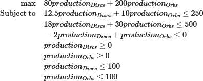
In addition, JuMP has an interesting feature that can output the model formulation in Latex format, as shown in Figure 6. The output lists every variable explicitly, rather than using an indexed style, so it is useful mainly for small models. Nonetheless, it can be helpful when checking that the model is specified as we intend.

Comparison between Julia/JuMP and Python/Pyomo

The Julia and Python programming languages have much in common. This is not a coincidence, as the designers of Julia adopted what they see as the best features of Python (and other languages) as part of the Julia design. Of course, there are differences in syntax, but there is enough broad similarity that learning Julia is not too difficult for a Python programmer.

For example, excluding the structural paraphernalia that's specific to each language, expressing a constraint in the two languages is almost identical, as shown in Figure 7.

sum(data.people[p] * production[p] for p in data.products) <= data.hours

sum(Model.People[p] * Model.Production[p] for p in Model.Products) <= Model.Hours

For this model, the Julia/JuMP program has 93 lines of code, while our equivalent Python/Pyomo program is a similar length, with 115 lines of code. The difference is not significant, with some things being easier in Julia, while others being easier in Python. In particular, the Julia/JuMP reporting functions are excellent.

Both Pyomo and JuMP provide access to a wide range of solvers. That's one reason why we prefer Pyomo over other Python libraries for most optimization models (the main exceptions being a preference for OR-Tools for constraint programming problems, and SciPy for non-convex global optimization problems). Helpfully, JuMP provides easy access to solvers via pre-configured packages that can simply be installed in Julia. Conversely, Pyomo requires some manual configuration to access solvers.

Julia is not yet as mature as Python, and the JuMP package has only recently achieved version 1.0 status. Python has many more libraries available, and a much larger user base makes it easier to find examples and support for Python compared with Julia. Even so, Julia and JuMP have all the essential aspects, and development continues to be active.

Overall, the combination of Julia/JuMP is a viable alternative to the more widely used Python tools.

Conclusion

We like the combination of Julia/JuMP. The syntax is sufficiently like Python/Pyomo that an experienced Python programmer should be able to learn Julia quickly.

Like Pyomo, JuMP has features specifically designed to facilitate the process of implementing an optimization model. The language syntax is clear and there are good tools that help the modelling process. Julia/JuMP is a strong contender for building optimization models. We think that Julia has the potential to become more widely adopted as an operational programming language over the next few years, as more people gain experience in the language.

If you would like to know more about this model, or you want help with your own models, then please contact us.