Solver Max - Python optimization Rosetta Stone

22 June 2022

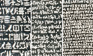
To start our exploration of optimization modelling in Python, we'll build the same linear programming model using several Python tools. We will, in a sense, develop a Rosetta Stone – with the same model translated into the different "languages" of the Python optimization modelling libraries. Our main purpose is to see how the libraries compare when applied to the same task.

Specifically, we'll replicate the linear program described in our article Production mix via graphical LP. That version of the Production mix model was built in Excel, using Solver/OpenSolver. In this series of articles, we'll build the Production mix model using the Python libraries:

Pyomo.
PuLP.
OR Tools.
Gekko.
CVXPY.
SciPy.

These are, as far as we're aware, the Python libraries that are most used for building linear programming models. Later, we'll add another library, Python MIP, when we use a variety of libraries to build mixed integer programming models.

Plan for this series of articles

In total, we'll build eleven versions of the Production mix model – all of which return the same solution, but using different libraries, solvers, and Python programming techniques.

Our first six models will be built using Pyomo, starting with a simple "concrete" model, progressing through a variety of increasingly sophisticated concrete models, ending with an "abstract" model. The range of Pyomo models illustrates some of the many techniques that can be used to build optimization models in Python, even when using the same library. We'll then build the Production mix model in each of the five other libraries.

In addition to using different libraries to build the models, some libraries have multiple solvers available. For each model, we'll choose an appropriate solver, depending on which solvers are available to the library we're using.

Articles in the Python Production mix series:

Our objectives

For this series of articles, our objectives are to:

Show how to build optimization models in Python.
Describe what the libraries have in common and how they differ.
Discuss the strengths and weaknesses of the libraries.

Some of the libraries are specifically designed for optimization modelling, while others have a wider scope. Therefore, we're particularly interested in which libraries are easy to use for the specific purpose of optimization modelling.

Situation

The Production mix situation is a typical small linear programming problem. That is, the situation we're modelling is:

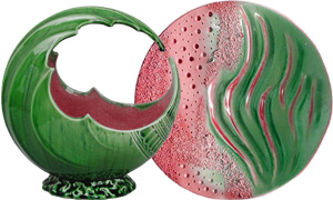
You own a boutique pottery business, making two types of large ornamental pieces: Lunar Orbs and Solar Discs (known succinctly as Discs and Orbs), as shown in Figure 1.
Your objective is to maximize gross profit margin per week.
You need to decide the number of units of Orbs and Discs to produce each week.
Production is constrained by staff hours, availability of materials, and experience about the number of units of each product that you can sell.

The sales experience constraint means that production of Orbs must be less than or equal to twice the production of Discs.

Mathematical formulation

We express the mathematical formulation in two ways:

General formulation. Uses general indices to represent data and variables.
Specific formulation. Replaces the indices with specific instances of the data and variables.

These two formulations are described in the following sections.

General formulation

When implementing a model, we usually start with a general formulation that describes the situation in mathematical notation.

The formulation for our Production mix model is shown in Figure 2, where the objective function and constraints are:

Equation (1). We want to maximize the total dollar profit margin from production.
Equation (2). The hours our people put into production must be less than or equal to the total hours available.
Equation (3). The use of materials must be less than or equal to the total kg of materials available.
Equation (4). Production of each product must be within limits derived from our sales experience.

Figure 2. General formulation

\begin{alignat}{1} &\text{Objective} \\ & \quad \text{Maximize} \ fTotalMargin &= \quad & \sum_{p=1}^n \text{dMargin}_{p} \times vProduction_{p} \tag{1} \\ \\ &\text{Subject to} \\ & \quad \sum_{p=1}^n \text{dPeople}_{p} \times vProduction_{p} &\le \quad & \text{dHours} \tag{2}\\ & \quad \sum_{p=1}^n \text{dMaterials}_{p} \times vProduction_{p} \quad &\le \quad & \text{dkg} \tag{3}\\ & \quad \sum_{p=1}^n \text{dSales}_{p} \times vProduction_{n} &\le \quad & 0 \tag{4}\\ \\ &\text{Variables} \\ & \quad vProduction_{p} &= \quad & \text{Units of each product} \quad &\forall \ p \in P \tag{5}\\ \\ &\text{Data} && \\ & \quad \text{dMargin}_{p} &= \quad &\text{Profit margin on each unit} \quad &\forall \ p \in P \tag{6}\\ & \quad \text{dPeople}_{p} &= \quad &\text{Staff hours to make each unit} \quad &\forall \ p \in P \tag{7}\\ & \quad \text{dMaterials}_{p} \quad &= \quad &\text{kg of materials to make each unit} \quad &\forall \ p \in P \tag{8}\\ & \quad \text{dSales}_{p} &= \quad &\text{Relative sales volume for each product} \quad &\forall \ p \in P \tag{9}\\ \\ &\text{Sets} \\ & \quad P &\ &\text{Product} \tag{10} \\ \\ &\text{Dimensions} \\ & \quad n &\ &\text{Number of products} \tag{11} \\ \\ &\text{Bounds} \\ & \quad \text{Non-negative} &\ &\quad \tag{12} \\ \end{alignat}

Note that the sales constraint (4), "production of Orbs must be less than or equal to twice the production of Discs", could be expressed as:

Production of Orbs <= 2 * Production of Discs

A more standard formulation is to move all variables to the left-hand side of the equation, leading to:

-2 * Production of Discs + Production of Orbs <= 0 (note the negative sign on the coefficient for Discs)

Equation (4) is the general form of this standard formulation.

Specific formulation

The general formulation states the structure of the situation that we're modelling. In our specific implementation, we have only two products: Discs and Orbs. Therefore, n=2 and the resulting model is quite simple. But we could, if necessary, expand the product range to any number of products without changing the general formulation.

In our specific situation, we have the following data:

The gross profit margin is $80.00 for each Disc and $200.00 for each Orb.
Production of a Disc requires 12.50 hours, and each Orb requires 10.00 hours.
Given the number of staff, and other commitments, a total of 250 staff hours are available for production each week.
Production of a Disc requires 18.00 kg of materials, and each Orb requires 30.00 kg of materials.
A total of 500 kg of materials is available each week.
The production of Orbs must be less than or equal to twice the production of Discs.

Therefore, our specific instance of the general formulation can be stated as shown in Figure 3, where Discs and Orbs are variables representing the number of each product that we make per week.

Figure 3. Specific formulation

\begin{alignat*}{1} &\text{Objective} \\ &\quad \text{Maximize}\quad\rlap{TotalMargin = 80.00 \times Discs + 200.00 \times Orbs} &&&&&&&\quad \quad \quad &\text{(13)}\\ \\ &\text{Subject to} \\ &\quad \phantom{-}12.50 \times Discs&{}+{}&10.00 \times Orbs&{} &\;\leq &\;&250 \quad \text{People, hours} &\quad &\text{(14)}\\ &\quad\phantom{-}18.00 \times Discs&{}+{}&30.00 \times Orbs&{} &\;\leq &\;&500 \quad \text{Materials, kg} &\quad &\text{(15)}\\ &\quad-2.00 \times Discs&{}+{}&\phantom{0}1.00 \times Orbs&{} &\;\leq &\;&\phantom{00}0 \quad \text{Sales} &\quad &\text{(16)}\\ \\ &\quad \rlap{Discs, Orbs \geq 0} &&&&&&&\quad &\text{(17)} \end{alignat*}

Template for Python optimization models

Given the mathematical formulations, we can proceed with implementing the model in Python. When writing Python code, our optimization models are generally divided into the following modules:

Import dependencies. Load the optimization library, along with any other libraries that we need for the program.
Get data. Import data from an external source, if applicable.
Declarations. Declare and populate data structures.
Define model. Specify the model's variables, constraints, and objective function.
Solve model. Solve the model, given options and a choice of solver.
Process results. Assess the outcome of the solve process and decide what output to write.
Write output. Write the model's solution, if there is one, or other output, if applicable.

Not all models require every module, and some larger or more complex models may require additional modules. Even so, we generally follow this consistent template, to make our models easier to understand, test, and modify.

Next steps

The next step is to implement the model in Python. We'll start by implementing the specific formulation, using the Pyomo library. Then we'll implement the general formulation in Pyomo, developing more sophisticated models along the way. After that, we'll implement the model in each of the other Python optimization libraries, to see how they differ.

For the first implementation, see the article Production mix - Model 1, Pyomo.

Python optimization Rosetta Stone