Set up a Python modelling environment

9 June 2022

A common issue encountered by new Python optimization modellers is setting up a Python environment. There are many libraries that can be used, and some – like Pyomo – require solvers to be installed separately. Getting everything working can be tricky and frustrating.

So, in this article we'll describe the steps we used to set up a new virtual environment, including Python, Jupyter Lab, several optimization modelling libraries, and a selection of solvers. We'll use this environment for subsequent blog articles about building and solving optimization models in Python.

We hope this article helps you create a working Python environment that enables you to replicate our models and build your own models. Note that we are using 64-bit Windows 10, so everything we do is in that context. If you are using a different operating system, then you'll need to adapt the instructions accordingly.

Overview of key setup steps

The key steps for setting up our Python modelling environment are:

• Install Python.
• Create a virtual environment.
• Install Jupyter Lab.
• Test Jupyter Lab.
• Install some other libraries.
• Install solvers for Pyomo.
• Complete setup of virtual environment.
• Test our environment by running a simple linear program.

Each of these steps is detailed in the following sections.

Setup steps

Install Python

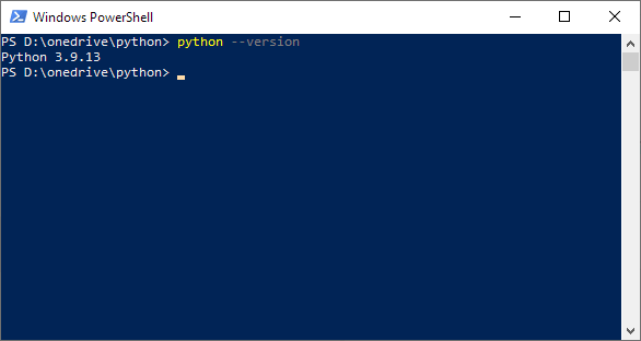
Your computer may already have Python installed. To test whether Python is installed, open a PowerShell window by clicking on the Windows Start button, typing PowerShell, and clicking on the app. Then, in PowerShell, type:

python --version

If your computer has Python installed, then the Python version will be displayed. For example, as shown in Figure 1, we have Python version 3.9.13 installed.

If the response is something like "'python' is not recognized as an internal or external command, operable program or batch file", then your computer does not have Python installed. To install Python, in a browser go to Python downloads and download a recent release of Python for your operating system. Open the installation application and then follow the instructions. After installing Python, check the Python version using the steps above.

Note that the specific Python version doesn't matter much – as long as it is fairly recent (i.e. version 3.8+). If your Python version is older, then just install a newer version, as described above. During the installation process, you should be asked to upgrade your existing version.

Create a virtual environment

You can use Python directly. But we want to have some control over our Python setup, so we will create a virtual environment. This enables us to keep our setup separate from any other Python installations on the same computer, which helps to avoid conflicts and incompatibility issues. To learn more about virtual environments, see Python virtual environments: A primer.

First, we need to create a start folder where the virtual environment will be installed. In our case, we create the folder D:\OneDrive\Python to contain everything associated with our Python blog articles.

Then, in PowerShell, we change to our start folder by typing cd d:\onedrive\python and pressing Enter. If you want, you can change PowerShell's start folder by editing its "Start in" property (right-click on the PowerShell icon, right-click on the Windows PowerShell task, and select Properties). If you do that, then PowerShell will start in that folder, so you won't need to change the folder every time you open PowerShell.

Our virtual environment needs a name – we'll call our environment blog. To create our virtual environment, in PowerShell (from your start folder) type the command:

python -m venv blog

That command creates the folder d:\onedrive\python\blog under the start folder, containing the files Python needs to operate a virtual environment.

To activate our virtual environment, we type the following command, which includes our folder's name:

blog\scripts\activate

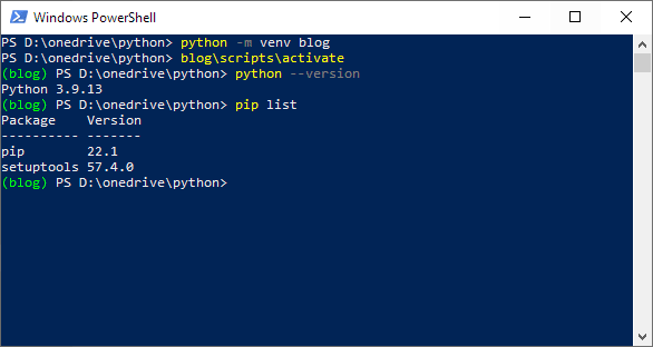
The PowerShell prompt should change to include the virtual environment's name, indicating that we're now working in our virtual environment. To check what our virtual environment contains, we can get the Python version by typing:

python --version

Then we can get a list of all installed packages using:

pip list

These steps are shown in Figure 2. Our virtual environment has Python version 3.9.13 and, since it is new, it has only two packages installed. You might be prompted to upgrade your version of pip – if so, then just follow the instructions provided when you call pip list.

Install Jupyter Lab

We'll be using a variety of libraries for our Python blog articles. A key library is Jupyter Lab, which is a web application for creating notebooks that can contain Python code and formatted documentation. Jupyter Lab is a good code development tool and notebooks are commonly used for sharing code.

To install Jupyter Lab, within the virtual environment, type:

pip install jupyterlab

It will take a while to install Jupyter Lab. Once it has finished, if you type pip list, then you'll see that the list of installed packages has expanded to several dozen, reflecting the wide range of Jupyter Lab's capabilities.

Test Jupyter Lab

Now that our virtual environment is set up and active, we start Jupyter Lab by typing in PowerShell:

jupyter-lab

Jupyter Lab will take control of the PowerShell window, then it will open a tab in the default browser. The tab should look something like Figure 3. The blog folder contains the files for the virtual environment. We will create other folders to contain our articles, solvers, documentation, etc.

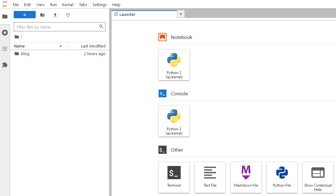
To test that Jupyter Lab works correctly, create a new notebook by clicking the Python 3 icon, or select File > New > Notebook.

A Jupyter Lab notebook consists of "cells", each of which can contain one of three types of content: programming code, markdown, or raw text. The type of content for the selected cell is shown in the toolbar, with the default being Code. We can create a simple Python program by typing in the first cell:

print('Hello world!')

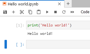
We execute the selected cell either by clicking the Run ▶︎ icon or pressing Shift+Enter. The result is shown in Figure 4. Python prints the text "Hello world!" below the cell, then creates a new cell ready for more content. Note that the number in square brackets, like [1], indicates the sequence in which the cells have been run.

The notebook is automatically saved in a file called Untitled.ipynb. You can rename the notebook by right-clicking on its name (either on its tab or in the navigation pane) and selecting Rename. You can also create a new folder and drag the file into that folder.

To close Jupyter Lab, just close the browser tab. If the PowerShell window doesn't close automatically, then close it.

Install some other libraries

We want to explore a variety of Python modelling tools in our blog articles, with the support of some general-purpose analysis and visualization tools. Specifically:

• cvxpy. A modelling language for convex optimization problems.
• gekko. Library for model construction, analysis, and visualization of simulation and optimization.
• matplotlib. General-purpose visualization and plotting library.
• mip. Collection of tools for the modeling and solution of mixed integer linear programs.
• numpy. Library of mathematical functions, random number generators, linear algebra routines, etc.
• ortools. Tools for modelling and solving combinatorial optimization problems.
• pandas. Library for data manipulation and analysis.
• pulp. Linear programming modelling library.
• pyomo. Library for building optimization models.
• scipy. A collection of algorithms and functions for conducting a wide range of modelling and analyses.

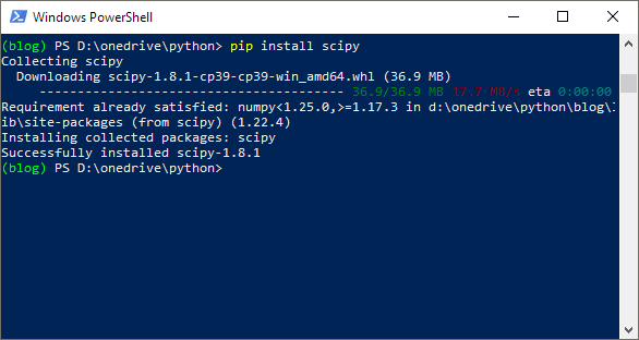
For example, to install scipy, open PowerShell, navigate to your virtual environment's start folder, and activate the virtual environment (as described above). Within the Python virtual environment, as shown in Figure 5, type:

pip install scipy

The scipy library will be installed under our d:\onedrive\python\blog folder.

Install the other libraries in a similar way, using the names in the list above – though numpy is installed with pandas, so we don't need to install it separately.

If there are other libraries you want to install, either now or later, then be sure to activate your virtual environment before installing them – otherwise they'll be installed outside the virtual environment, so they won't be available inside the environment.

To close the virtual environment, either type deactivate at the prompt (so that you can continue working in PowerShell) or, if you're finished working with both the virtual environment and PowerShell, then simple close the PowerShell window.

Install solvers for Pyomo

Most of the modelling libraries have solvers built in. An exception is Pyomo, which is a modelling tool that can call a variety of solvers, but it has none installed by default.

So, let's install some solvers for Pyomo, specifically:

• Bonmin (Basic Open-source Nonlinear Mixed INteger programming). For convex and non-convex non-linear mixed integer models.
• CBC (COIN-OR Branch-and-Cut). For continuous and integer linear models.
• Couenne (Convex Over and Under ENvelopes for Nonlinear Estimation). A global optimizer for mixed integer non-linear optimization models.
• GLPK (GNU Linear Programming Kit). For continuous and integer linear models.
• IPOPT (Interior Point OPTimizer). For continuous and integer non-linear models.

CBC, Bonmin, and Couenne are also available in the Advanced version of OpenSolver for Excel, which we use for some other blog articles.

We'll start by installing GLPK:

• Made a new folder in the virtual environment's start folder, like D:\onedrive\python\solvers.
• Made a new sub-folder specifically for GLPK, like D:\onedrive\python\solvers\glpk.
• Download the latest version of GLPK from https://sourceforge.net/projects/winglpk.
• Unzip the downloaded file.
• Since we're using Windows 64-bit, copy the contents of the extracted w64 folder to the newly created sub-folder glpk.
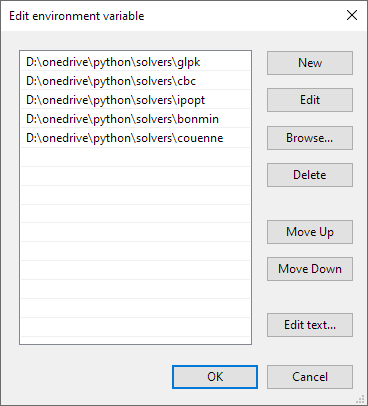
• Put the full path of the glpk folder on the operating system's user path (use the Windows search feature to find "Edit the system environment variables", then select Environment variables > User variables > Path Edit > New).

To install the other solvers, download the appropriate binary file for each of Bonmin, CBC, Couenne, and IPOPT from the AMPL website. Put the downloaded files in separate sub-folders like we did for glpk. Then add each of those folders to the Windows path.

Figure 6 shows the list of solver folders in the Windows path variable. You may also have other existing entries in the path list – leave those unchanged.

Note that, although we placed the solvers under the virtual environment's start folder, access to the solvers is not restricted only to the virtual environment as the Windows path variable makes the files accessible from anywhere.

Complete setup of virtual environment

If Jupyter Lab is open when folders are added to the Windows path, then Jupyter Lab will not recognize the solvers in those folders. So, if Jupyter Lab was open when you made changes to the path, you need to close Jupyter Lab, close the virtual environment, re-activate the virtual environment, and then re-start Jupyter Lab (using the instructions above).

Everything should now be ready, so let's test that it works.

Test our environment by running a simple linear program

Finally, let's run a simple linear program in Jupyter Lab. The Production mix model is contained in the notebook below (right-click and select Save Link As, rather than opening the file in the browser).

Download the notebook production-mix-1.ipynb

Save the notebook to a sub-folder of your virtual environment's start folder. For example, we created a folder called Articles, so we put the file in a sub-folder called Python setup, resulting in the full file path D:\OneDrive\Python\Articles\Python setup\production-mix-1.ipynb.

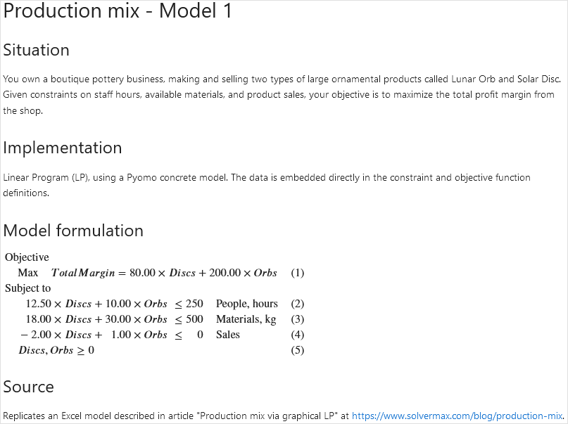
Start Jupyter Lab and navigate to the folder where you put the notebook. The notebook file should appear in the file browser on the left of the Jupyter Lab tab. Open the notebook – the first cell contains some documentation for the model, in Markdown format, as shown in Figure 7.

The model's Python code in shown in Figure 8.

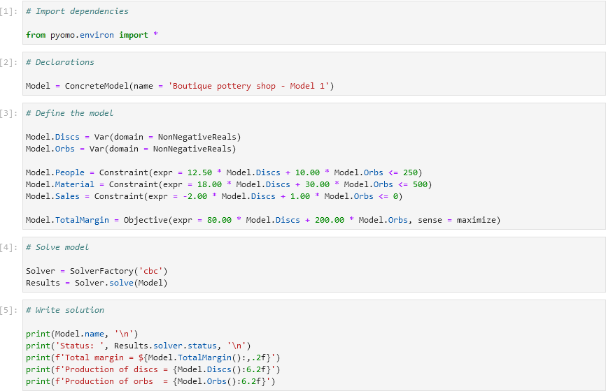
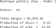
Run each cell in sequence, starting by selecting the first (documentation) cell and then clicking the Run ▶︎ icon six times (or select the first cell and click the Run All ▶︎▶︎ icon). The output should look like Figure 9, which shows the model's solution.

This notebook is a Python implementation, using Pyomo and the CBC solver, of the model we built using Excel in our blog article Production mix via graphical LP. The solution shown in Figure 9 is the same as the optimal solution we found using OpenSolver in Excel.

A key feature of Pyomo is that we can easily change the solver that it uses. As a test, edit the line that specifies that Pyomo uses the CBC solver:

Solver = SolverFactory('cbc')

Change the line to use the GLPK solver instead:

Solver = SolverFactory('glpk')

We don't need to re-run the cells before the one we edited, so select the cell we edited and click the Run icon twice (to run that cell and the next cell that writes the output). The output should be the same, though this time we solved the model using GLPK rather than CBC.

Conclusion

All going well, you should now have a working Python virtual environment in which you can solve optimization models in Jupyter Lab notebooks.

In the next article, we'll start a series of articles that explore different features of the Pyomo and other optimization modelling libraries. We'll use the Production mix model as a example – we'll see how the code works, and also expand and improve it in a variety of ways.

If you would like to know more about setting up a Python optimization environment, or you want help with your own models, then please contact us.