16 November 2021

Recently we were working on a small one-dimensional bin packing model. The situation was simple, and we expected the model to be easy to solve. But there was just one problem: we couldn't find an optimal solution, even after letting the solver run overnight for 12 hours.
Initially, we were using the CBC solver. Since that didn't work, we tried CPLEX via NEOS, but we encountered the same problem – CPLEX couldn't find an optimal solution either.
So, we searched the Operations Research literature for an alternative formulation. We discovered a recently published academic paper that has a new, innovative formulation for one-dimensional bin packing (and potentially other types of packing situations).
This article describes the new formulation and our experience applying it to our simple, yet difficult to solve, model.
Download the model
The model is available on GitHub.
Situation
We have 50 items that we want to pack into as few bins as possible. Each item has the same width and depth, which match the width and depth of the bins, but different heights that vary potentially from 500 to 1,500 units. Each bin has a height of 3,000 units. That is, we have a one-dimensional bin packing problem.
Only a small number of items will fit in each bin – potentially between 2 and 6 items per bin (i.e. 3,000 / 1,500 and 3,000 / 500 respectively). If the items are not allocated to bins efficiently, then we may have a lot of unused bin capacity, which is what we are trying to avoid.
The total height of our 50 items is 50,903 units, which equates to 50,903 / 3,000 = 16.97 bins. Therefore, we need at least 17 bins. If we can fit the 50 items into 17 bins, then the packing will be very tight. Given the specific items that we need to pack, 17 bins might not be feasible. Instead, we might need to use 18 (or more) bins.
Model 1
Model 1: Design
Conventional model formulation
We start with a conventional formulation for the one-dimensional bin packing problem, as shown in Figure 1. That is:
- Equation (1). We want to minimize the number of bins used.
- Equation (2). All items must be allocated to a bin.
- Equation (3). If a bin is used, then the total height of items allocated to that bin must be less than or equal to that bin's capacity.
- Equation (4). We want to allocate each item to a bin, so we have an Items by Bins matrix of binary variables.
- Equation (5). We have binary variables to indicate which bins are used.
Model 1: Implementation

Allocate items to bins
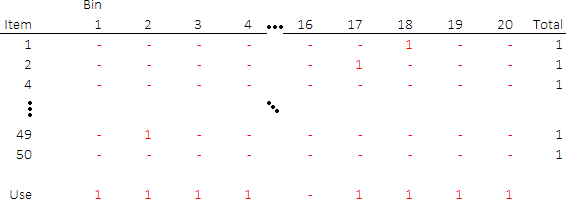
The essence of this formulation is encoded in the meaning of the two sets of variables, parts of which are shown in Figure 2. That is, we have binary variables to indicate which bins to use, and binary variables to indicate allocation of items to bins.
For example, the solution shown allocates Item 1 to Bin 18, and it uses Bin 1 but it doesn't use Bin 16, etc.
As we calculated above, the items need at least 17 bins. To provide some flexibility, we allow the solver to use up to 20 bins. With 50 items and 20 bins, our allocation matrix has 50 * 20 = 1,000 variables. The model has an additional 20 variables representing the bins.
Pack the items within the bin capacity

All our bins have the same capacity – though in a more general situation that is not necessarily the case.
As shown in Figure 3, we calculate the height of all items allocated to a bin, then constrain that total height to be no more than the height of that bin.
Note that if a bin is not used, for example Bin 16, then its available capacity is zero. This ensures that no items are allocated to an unused bin.
Model 1: Solver model
Objective function
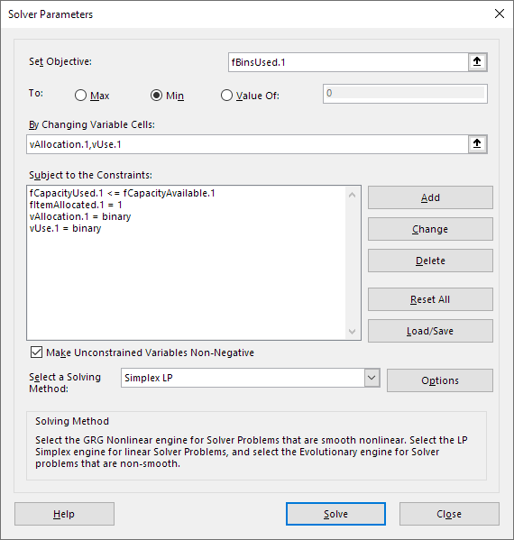
The Solver model is shown in Figure 4. Our objective is to minimize fBinsUsed.1. Note that the range name includes the suffix .1, which we use to indicate that this range name is local to the Model 1 worksheet, to distinguish it from range names for other model worksheets.

Variables
The model has two sets of variables:
vAllocation.1. Allocation of items to bins.vUse.1. Whether a bin is used.
Constraints
The constraints are:
fCapacityUsed.1 <= fCapacityAvailable.1. For each bin, the used capacity must be no more than the capacity available.fItemAllocated.1 = 1. All items must be allocated to a bin.vAllocation.1 = binary. The allocation variables are binary.vUse.1 = binary. The use variables are binary.
Solution method
Our model is too large for Solver, so we use the CBC solver via OpenSolver.
Model 1: Analysis
Optimal solution
Although our model is simple and reasonably small, the CBC solver fails to find an optimal solution in a reasonable time.
That is, CBC takes a few seconds to find a solution that uses 18 bins. But after an hour, CBC has not found a proven optimal solution. We then let CBC run for 12 hours, but it makes no further progress.
Making use of the procedure described in our article We need more power: NEOS Server, we try using the more powerful CPLEX solver. However, CPLEX also fails to make any progress beyond a solution that uses 18 bins (which it found after a few seconds).
After an hour of run time, the best solution found by CPLEX is shown in Figure 5. For presentation, we have sorted the bins in decreasing order of remaining available capacity.
In this solution, our 50 items are packed into 18 of the 20 available bins, with a significant amount of available capacity remaining in some of the used bins. We had hoped that the items could be packed into 17 bins, though we still don't know if that is feasible – CPLEX hasn't found a solution with 17 bins, but it also hasn't proven such a solution to be infeasible. Note that there are many alternative solutions that use 18 bins.
Model 2
Model 2: Design
Our Model 1 formulation works, but we can't find an optimal solution – even when using the CPLEX solver. Time to try a different approach.
Model 1 uses a conventional one-dimensional bin packing formulation. But there are often many ways to design an optimization model formulation. So, we searched the web for ideas about how we could modify our formulation to improve performance.
Most of the search results were either heuristics or mixed integer linear program formulations that are essentially the same as Model 1. However, an academic paper from a conference in 2020 caught our attention: "New Symmetry-less ILP Formulation for the Classical One Dimensional Bin-Packing Problem" (the full reference is provided at the end of this article, including a link to the paper).
This new formulation takes a radically different approach to bin packing. As shown in Figure 6, unlike Model 1, the new formulation does not explicitly represent the bins. Instead, it allocates items using an Items by Items matrix of binary variables, where the main diagonal of the matrix implicitly represents the bins.
In addition, like for Model 1, this model has constraints that require each item to be allocated, and the total capacity allocated to an implicit bin must be no more than the bin's available capacity.
Model 2: Implementation

Allocate items implicitly
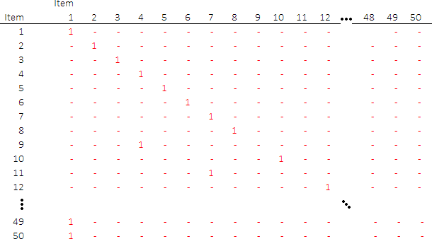
Figure 7 shows part of the allocation matrix for Model 2.
With 50 items, the allocation matrix is 50 by 50, so there are 2,500 variables in this matrix. This is much larger than the 1,000 variables in Model 1's allocation matrix.
Interpretation of the allocation matrix implies three regions:
- The main diagonal implicitly represents the bins.
- All variables in the lower-left triangle of the allocation matrix are allocated to the same bin as the item on the main diagonal in that column.
- All variables in the upper-right triangle of the allocation matrix must be zero. Therefore, we ignore those variables in the constraints.
The source paper describes this formulation in more detail. It is worthwhile reading the paper, to better understand the thinking behind the design of this formulation.
Model 2: Solver model
Objective function
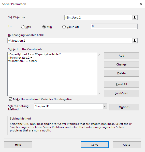
The Solver model is shown in Figure 8. Our objective is to minimize fBinsUsed.2, which is the sum of variables on the main diagonal of the allocation matrix.

Variables
The model has only one set of variables:
vAllocation.2. Allocation of items.
Constraints
The constraints are:
fCapacityUsed.2 <= fCapacityAvailable.2. For each bin, the used capacity must be no more than the capacity available.fItemAllocated.2 = 1. All items must be allocated.vAllocation.2 = binary. The allocation variables are binary.
Model 2: Analysis
Optimal solution
CBC also struggles with this model, so from here onwards we just use CPLEX.
Surprisingly, given our difficulty in finding an optimal solution with Model 1, CPLEX solves Model 2 to optimality in a few seconds.
As shown in Figure 9, the optimal solution uses 17 bins – one bin less than we were able to find using Model 1. As expected, the packing is very tight, with little or no available capacity remaining in the used bins.
Model 3: Design
The source paper extends Model 2 by proposing two additional cutting plane constraints that are designed to reduce the size of the model's solution space. The paper's authors report mixed success in applying the cuts. Cut 2 is simpler, and it seems to be tighter, so we try Cut 2 to see if it improves the performance of our Model 2.
The formulation for Cut 2 is shown in Figure 10. This constraint is simply added to Model 2.
Model 3: Analysis
Performance impact of Cut 2
Adding Cut 2 to Model 2 significantly increases the model size. In this example, the additional constraint also increases the time to find an optimal solution – taking 5.4 seconds, compared with 2.6 seconds for Model 2.
Testing the models on additional cases
Run each model with different items
Our reason for seeking an alternative formulation was that CPLEX failed to solve our conventional formulation to optimality in a reasonable time. Conversely, the new symmetry-less formulation works splendidly, solving our bin packing problem to optimality in a few seconds.
However, so far, we've tried the new formulation on only one set of data. While the paper's authors are enthusiastic about their new formulation, they report some examples where the new formulation performs worse than a conventional formulation.
To see how the formulations compare in our situation, we ran each model with nine additional cases. That is, bin capacity of 3,000 and 50 randomly generated items with sizes between 500 and 1,500 (the data for each case is available in the attached spreadsheet). The results are shown in Figure 11, where Case 1 is the data that we have been using up until this point.
In comparing the formulations, we're interested in the time to find a proven optimal solution. These cases demonstrate some clear patterns:
- In half the conventional formulation (Model 1) cases, CPLEX failed to find a proven optimal solution within one hour of run time (as indicated by an "x" in the run time). In addition, the run time for Case 6 was almost 34 minutes.
- The cases where Model 1 failed all have an unrounded lower bound that is close to the next integer. That is, if the lower bound is feasible, then the packing will be tight. For example, Case 1 has an unrounded lower bound of 16.97. So, packing the items into 17 bins (if possible, which it turns out it is) will leave little available capacity in the used bins.
- For all cases, the new formulation (Model 2) found a proven optimal solution in a few seconds.
- Model 2 is faster than Model 1 in all cases, though in the cases where the packing isn't tight the run time difference is small.
- For all cases, the new formulation with Cut 2 (Model 3) found a proven optimal solution in a few seconds, though it is slower than Model 2 in all but one case (Case 2).
- Except for Cases 8 and 9, the optimal solutions are equal to the rounded up lower bound.
In our situation, the new formulation, Model 2, performs much better than the conventional formulation, Model 1. However, including Cut 2 is not worthwhile in this situation.
Conclusion
This article demonstrates the value of exploring alternative model formulations. Although the one-dimensional bin packing problem has been researched for decades, advances in the state-of-the-art continue to occur.
We started with a simple situation and a conventional formulation. But our first model didn't work well, given the tight packing implied by our data. Adopting a new, recently published, formulation has enabled us to substantially improve the model's performance, so that the problem can now be solved to optimality quickly for a variety of data sets.
If you would like to know more about this model, or you want help with your own models, then please contact us.
References
Models 2 and 3 are based on the paper:
Salem, K. H., & Kieffer, Y. (2020). "New Symmetry-less ILP Formulation for the Classical One Dimensional Bin-Packing Problem". In Kim D., Uma R., Cai Z., Lee D. (editors), Computing and Combinatorics, 26th International Conference, August 2020, pp. 423-434.
