Solver Max - Facility location optimization in Excel

25 January 2021

The "facility location problem" is a common, and often difficult, decision that organizations need to make.

Facilities may include assets such as factories, warehouses, shops, mobile telephone sites, etc. Such assets are typically long-lived, so the decision about where to build them has a long-term impact on the organization.

A wrong, or sub-optimal, decision is likely to be very expensive. To help make the decision, we can model the facility location problem using an optimization model in Excel.

Download the models

The model is available on GitHub.

Situation

We operate a business that serves customers from local facilities. We are looking to expand our business into a new region, so we need to decide how many facilities to build and where to build them within the region.

Our objective is to maximize annual profit from operating in the new region.

Model design

Potential approaches to selecting locations

There are numerous approaches to modelling facility location problems.

For example, we may have a list of specific sites where facilities could be located. Our model can select the facilities from the list that maximize the expected profit in the region.

A more general approach is to divide the region into a grid of areas where facilities may be located. We then designate which surrounding areas can be serviced by each facility. Our model can then choose the combination of areas that maximize the expected profit.

Divide the region into a grid

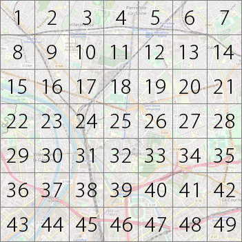
Regional map as a grid — Figure 1. Regional map as a 7x7 grid

In this situation, we'll take the latter approach. Specifically, a map of the new region is divided into a grid of 7x7 areas, as shown in Figure 1. A facility can serve the customers in the 3x3 block centered on its area. For example, a facility in area 25 can serve areas 17, 18, 19, 24, 25, 26, 31, 32, and 33.

We're using a small grid to keep the model size small, but we could increase the model's resolution by using a grid with more (smaller) areas. The model formulation would be the same if we used more areas, though more input data would be required and the solution time may increase significantly.

Define the data we need for the model

We need to analyze the characteristics that we care about in each area of the grid, so we can decide which areas are best. In this situation, we estimate:

Build cost, expressed as an annualized amount, if a facility is built in that area.
Operating cost, per annum, if a facility is built in that area.
Area revenue, per annum, if at least one facility provides coverage to serve that area.

We express all the data on a consistent annual basis for simplicity. An alternative approach would be to calculate the Net Present Value of costs and revenues over an appropriate time horizon. That approach would not fundamentally change the model, though it is more complex to implement.

In addition, there are two assumptions that we can use to control the solution process. These will enable us to do some analyses that enhances our understand of the model's behavior, and so they help us make the facility location decision:

Coverage required. We may want to mandate the minimum number of facilities serving each area. Zero means that the model will decide.
Must build. To help us understand how the model behaves as the number of facilities changes, we want the ability to specify the total number of facilities to build. Zero means that the model will decide.

Formulation

The mathematical formulation for our model is shown in Figure 2. That is:

Equation (1). Maximize the annualized profit from all cells in the region.
Equation (2). The number of facilities built must be at least a specified lower bound.
Equation (3). The number of facilities built must be no more than a specified upper bound.
Equation (4). The facilities must provide at least the required coverage in each cell.
Equation (5). A cell has coverage if a facility is built in an adjacent cell.

Figure 2. Mathematical formulation

\begin{alignat*}{1} &\text{Objective} \\ &\quad \text{Min } fProfit &=\quad &\sum_{x=1}^m \sum_{y=1}^n \left( \text{dRevenue}_{x,y} \times vHasService_{x,y} \right) \\ &&&- \sum_{x=1}^m \sum_{y=1}^n \left( \text{dBuildCost}_{x,y} \times vBuild_{x,y} \right) \\ &&&- \sum_{x=1}^m \sum_{y=1}^n \left( \text{dOperatingCost}_{x,y} \times vBuild_{x,y} \right) \tag{1} \\ \\ &\text{Subject to} \\ &\quad \sum_{x=1}^m \sum_{y=1}^n vBuild_{x,y} &\ge \quad & \begin{cases} 0, \text{if dMustBuild = 0} \\ \text{dMustBuild}, \text{otherwise} \end{cases} \tag{2} \\ & \quad \sum_{x=1}^m \sum_{y=1}^n vBuild_{x,y} &\le \quad & \begin{cases} \lvert \text{dBuildCost} > 0 \rvert, \text{if dMustBuild = 0} \\ \text{dMustBuild}, \text{otherwise} \end{cases} \tag{3} \\ &\quad \sum_{x-1}^{x+1} \sum_{y-1}^{y+1} vBuild_{x,y} &\ge \quad &\text{dCoverageRequired} &\forall \ x \in X, \forall \ y \in Y \tag{4}\\ &\quad \sum_{x-1}^{x+1} \sum_{y-1}^{y+1} vBuild_{x,y} &\ge \quad &vHasService_{x,y} &\forall \ x \in X, \forall \ y \in Y \tag{5}\\ \\ &\text{Variables} \\ &\quad vHasBuild_{x,y} &= \quad & \begin{cases} 1, \text{if build in cell $x,y$} \\ 0, \text{otherwise} \tag{6} \end{cases} &\forall \ x \in X, \forall \ y \in Y \\ &\quad vHasService_{x,y} &= \quad & \begin{cases} 1, \text{if count of facilities in 3x3 block} \\ \quad \text{centered on cell $x,y$ is $\ge$ 1} \\ 0, \text{otherwise} \tag{7} \end{cases} &\forall \ x \in X, \forall \ y \in Y \\ \\ &\text{Data} \\ &\quad \text{dCoverageRequired} \ \ &= \quad &\text{Positive integer, facilities} \tag{8} \\ &\quad \text{dMustBuild} &= \quad &\text{Positive integer, facilities} \tag{9} \\ &\quad \text{dRevenue}_{x,y} &= \quad &\text{Positive real, \$/year} &\forall \ x \in X, \forall \ y \in Y \tag{10}\\ &\quad \text{dBuildCost}_{x,y} &= \quad &\text{Positive real, \$/year} &\forall \ x \in X, \forall \ y \in Y \tag{11}\\ &\quad \text{dOperatingCost}_{x,y} &= \quad &\text{Positive real, \$/year} &\forall \ x \in X, \forall \ y \in Y \tag{12}\\ \\ &\text{Sets} \\ &\quad X &\ &\text{Horizontal grid position} \tag{13} \\ &\quad Y &\ &\text{Vertical grid position} \tag{14} \\ \\ &\text{Dimensions} \\ &\quad m &\ &\text{Number of horizontal cells} \tag{15} \\ &\quad n &\ &\text{Number of vertical cells} \tag{16} \\ \\ &\text{Bounds} \\ & \quad \text{Non-negative} &\ &\quad \tag{17} \\ \end{alignat*}

Implementation

Build costs — Figure 3. Build cost in each area

Technique for avoiding special cases

A consequence of representing the region as a grid is that we create special cases around the edges and corners.

Specifically:

In the middle of the region, each area serves a 3x3 block of areas.
An edge area can serve only 6 areas.
A corner area can serve only 4 areas.

To avoid having to deal with the special cases, we extend the grid so that it is surrounded by a fringe of hard-coded zeros. This enables consistent formulae to be used for all areas, as each area can now "serve" a full 3x3 block of areas, though around the edges and corners some areas always have zero values.

This technique for handling special cases on the edge of data sets is applicable to a wide range of models. It reduces the complexity of the implementation and make the model easier to understand and change.

Specifying our data

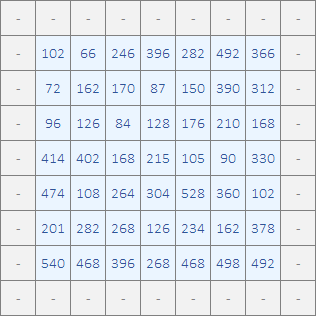
Figure 3 shows a 7x7 block of cells, plus the surrounding fringe of hard-coded zero values, that are our estimated annualized Build cost per area.

There are similar blocks of data for the annual Operating cost and expected potential Area revenue from each area.

The annualized build costs vary substantially from area to area. Some areas have a relatively low cost, so they may be attractive areas to build a facility – though that decision also depends on the operating cost in that area and the expected revenue from that area and the surrounding areas.

Conversely, some areas have high build costs, particularly around the northeast, southeast, and southwest corners. Since our objective is to maximize profit, the model will tend to avoid these high-cost areas – unless they are sufficiently compensated by low operating costs and/or high expected revenue.

Specify where the model can make build decisions

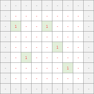
The Build decision for each area is represented as a binary variable, where 1 means build in that area and 0 means don't build in that area.

An example block of build decisions is shown in Figure 4, where the solution is to build 5 facilities in the highlighted areas.

The model can choose to build only within the 7x7 grid of areas; it cannot build in the surrounding fringe.

Calculate the coverage achieved by the build decisions

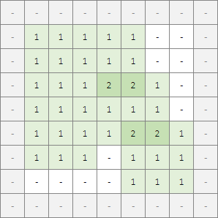
Given the build decisions, we can calculate the area coverage, as shown in Figure 5.

The coverage calculation sums the Build decisions in a 3x3 block around each area. Because we've included the fringe, the calculation for every area is the same, which simplifies the formulae.

Build coverage — Figure 5. Coverage from the build decisions

Points to note:

Some areas are covered by more than one facility. For example, area 18 has coverage of 2, being served by the facilities built in areas 11 and 26.
Other areas, in and around the northeast and southwest corners, have no coverage due to their high build costs and low potential revenue.
Areas in the southeast corner also have high build costs, but we can cover those areas by building in the adjacent area 41.

Solver model

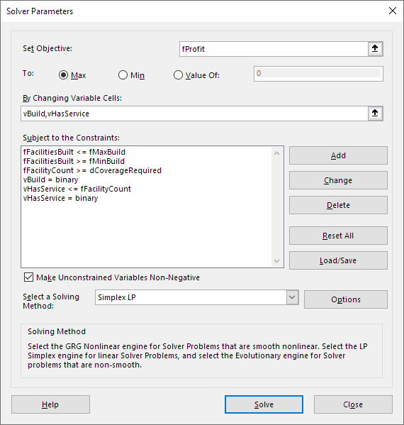
The Solver model is shown in Figure 6.

Objective function

Our objective is to maximize fProfit, which is calculated as the sum over all areas of:

Revenue from areas that have coverage minus (Build cost plus Operating cost).

Variables

The model uses two sets of binary variables:

vBuild. A 7x7 block that indicates the build decision in each area, as shown in Figure 4. If this variable has a value of 1 in an area, then the Facility build cost and Facility operating cost in that area are included in the objective function.
vHasService. A 7x7 block that indicates if an area is serviced by at least one facility, either in that area or from an adjacent area. If this variable has a value of 1 in an area, then the Area revenue is included in the objective function. We use this variable, rather than the count of facilities serving the area, because the revenue from an area does not change if it is served by more than one facility.

Constraints

fFacilitiesBuilt <= fMaxBuild. Defines the maximum number of facilities that can be built.
fFacilitiesBuilt >= fMinBuild. Defines the minimum number of facilities that can be built.
fFacilityCount >= dCoverageRequired. Specifies how many facilities must serve each area. If the Coverage required assumption is zero, then the model may choose to not provide service to an area, otherwise the model must provide at least the specified coverage.
vBuild = binary. The build choice in each area is binary (1 = build, 0 = don't build).
vHasService <= fFacilityCount. Ensures that the vHasService variable for an area equals 1 only if that area is covered by at least one facility (otherwise it equals 0). If an area has service, then it produces the Area revenue assumed for that area. Having multiple facilities servicing an area does not change the revenue from that area.
vHasService= binary. An area either has service, or it doesn't.

The vBuild and vHasService variables are related via a calculation of the number of facilities that cover each area, fFacilityCount, which sums each 3x3 block shown in Figure 4 (including, for the edges and corners, the fringe areas outside the 7x7 grid).

The Must build assumption defines how the fFacilitiesBuilt constraints behave:

If the Must build assumption is zero, then fMinBuild is set to zero and fMaxBuild is set to the number of areas in the grid – so the number of facilities to build is effectively unconstrained.
If the Must build assumption is non-zero, then both fMinBuild and fMaxBuild are set to the assumption – so the number of facilities to build must equal the assumption. That is, in general, the combination of constraints like x >= y and x <= y is equivalent to the single constraint x = y.

Solution method

This model is a Mixed Integer Program (MIP), so it can be solved efficiently using the Simplex method. The model can be solved by either Solver or OpenSolver. The model is quite small and the solver can find an optimal solution quickly, so the run time is only a few seconds.

Analysis

Optimal solution

Given our data and constraints, the optimal solution is to build 5 facilities in the areas shown in Figure 3. The resulting profit from the region is $1,794,000 per annum.

This optimal profit is also shown as the highest point on the chart in Figure 7. An "inverted U" shape is typical for many types of maximization model.

Figure 7. Range of solutions for various assumptions

Effect of varying the number of facilities built

We can explore the solution space by varying the Coverage required and Must build assumptions.

First, we set Coverage required to 0, so the model can decide what coverage to use for each area. Then we incrementally set the Must build assumption to each integer from 0 to 15 and solve for the optimal build.

The profit results are shown as the blue series of dots on the chart, indicating how the optimal solution varies depending on the number of facilities built:

With only a few facilities, we can increase profit by building more facilities to capture more of the potential revenue available in the region.
Beyond 5 facilities, we start incurring costs that are not sufficiently reimbursed by the marginal revenue – mainly because we are covering many of the same areas that are already covered by other facilities.
Building 15 facilities results in a small loss overall. Beyond 15 facilities, the loss continues to increase.

Note that the blue dots represent only the optimal solution for each number of facilities built. There are many other sub-optimal solutions. For example:

If we tell the model that it must build exactly one facility, then there are only 49 possible solutions – corresponding to each of the 7x7 areas in the grid.
But if we tell the model that it must build exactly 24 facilities (that is, in around half the areas), then there are 63 million million possible solutions. This is the number of combinations of 24 items from 49 possibilities, where the order doesn't matter and the items cannot be repeated. In Excel, this value is calculated using the formula =COMBIN(49,24).

The fact that we can solve this model to optimality in a few seconds illustrates the power of this type of modelling.

Effect of requiring full coverage

Similarly, we can repeat the analysis with the Coverage required assumption set to 1. This forces the model to ensure that every area is served by at least one facility. We may want to do this to see the impact of providing full coverage of all areas in the region.

The result, as shown by the orange series of dots on the chart, is that we would need to build at least 9 facilities. With our 7x7 grid, it is not feasible to cover all areas with fewer than 9 facilities. Because we must cover every area, the model is forced to build facilities near the expensive northeast and southwest corners, where it previously chose not to build. Forcing the model to build in those areas significantly reduces profit.

Conclusion

This model is a simple, though powerful, example of solving a facility location problem in Excel.

Given our assumptions, the model finds the optimal number of facilities and their best locations within the region. By including assumptions to control the solution process, we can do additional analyses that give us further insight into the situation. These insights enable us to make a more informed decision about where to locate our facilities.

If you would like to know more about this model, or you want help with your own models, then please contact us.

Facility location optimization in Excel