Solver Max - On the shoulders of giants

15 March 2021

Designing an optimization model can be difficult. In seeking guidance, we often look for inspiration from the published academic literature. Since the 1950s, there has been an enormous amount of research into how to design and solve optimization models for a wide range of situations, with models for just about anything we could want.

There is much that we can learn from the literature, if only we could understand it. Many academic papers include a statement of the model's design, known as the formulation, using mathematical notation that can look impenetrable. The notation is seldom explained, so translating a formulation into a working model can be a perplexing and frustrating process.

But with a little knowledge about what the notation means, we can gain a lot of insight into how to design or improve our models. The purpose of this article is to explain the meaning of common mathematical notation and illustrate how we can apply the knowledge contained in academic papers to help us build working models in Excel.

Download the models

The model is available on GitHub.

Situation

To illustrate how we can translate a model's mathematical formulation into Excel, suppose we have the following situation:

We want to allocate people to desks in an office.
Each person has indicated a preference for each desk, using a score from 1 = low preference to 10 = high preference.
The number of desks equals the number of people.
A desk may not be available to a person.
We want to maximize the total of the preference scores that result from our allocation decisions.

Model design

Mathematical formulation

Figure 1 shows the mathematical formulation for our model, in a style like that used in academic papers.

There are many different notation conventions adopted by different authors and publications. Such diversity can make it difficult to interpret the equations. Even so, there is sufficient commonality that we usually can decipher the intended meaning of the formulation.

Figure 1. Our model's mathematical formulation

\begin{alignat}{1} &\text{Objective} \\ & \quad \text{Maximize} \ fScore &= \quad &\sum_{p=1}^m \sum_{d=1}^n \left( \text{dPreference}_{p,d} \times vAllocation_{p,d} \right) \tag{1} \\ \\ &\text{Subject to} \\ & \quad \sum_{p=1}^m vAllocation_{p,d} \ \ &= \quad &1 \tag{2} &\begin{array}{l} \forall \ d \in \{1 \ldots n\} \\ \end{array} \\ & \quad \sum_{d=1}^n vAllocation_{p,d} &= \quad &1 \tag{3} &\begin{array}{l} \forall \ p \in \{1 \ldots m\} \\ \end{array} \\ & \quad vAllocation_{p,d} &\leq \quad &\text{dAvailability}_{p,d} \tag{4} &\begin{array}{l} \forall \ p \in \{1 \ldots m\} \\ \forall \ d \in \{1 \ldots n\} \\ \end{array} \\ \\ &\text{Variables} \\ & \quad vAllocation_{p,d} &= \quad &\begin{cases} 1, &\text{if person \(p\) is allocated to desk \(d\)} \\ 0, &\text{otherwise} \tag{5} \end{cases} &\begin{array}{l} \forall \ p \in \{1 \ldots m\} \\ \forall \ d \in \{1 \ldots n\} \\ \end{array} \\ \\ &\text{Data} && \\ & \quad \text{dAvailability}_{p,d} &= \quad &\begin{cases} 1, &\text{if desk \(d\) is available to person \(p\)} \\ 0, &\text{otherwise} \tag{6} \end{cases} &\begin{array}{l} \forall \ p \in \{1 \ldots m\} \\ \forall \ d \in \{1 \ldots n\} \\ \end{array} \\ & \quad \text{dPreference}_{p,d} &= \quad \tag{7} &\begin{array}{l} \text{Person \(p\) preference for desk \(d\)} \\ \text{(1 low \(\ldots\) 10 high)} \end{array} &\begin{array}{l} \forall \ p \in \{1 \ldots m\} \\ \forall \ d \in \{1 \ldots n\} \\ \end{array} \\ \\ &\text{Indices} \\ & \quad p &\ & \text{Person} \tag{8} \\ & \quad d &\ & \text{Desk} \tag{9} \\ \\ &\text{Dimensions} \quad \\ & \quad m &\ & \text{Number of people} \tag{10} \\ & \quad n &\ & \text{Number of desks} \tag{11} \\ \\ &\text{Bounds} \\ & \quad \text{Non-negative} &\ &\quad \tag{12} \\ \end{alignat}

The formulation consists of the following sections:

Objective. Specifies the objective function and whether we want to minimize or maximize that function.
Subject to. Specifies the constraints that the objective function is subject to.
Variables. Defines the variables for our model.
Data. Defines the data that is input to the model.
Indices. Defines the indices, or sets, for the data, variables, and constraints.
Dimensions. Defines the dimensions of the sets.
Bounds. Allow variables to be free (negative or positive), or be non-negative.

Notation used in the formulation

To aid with interpretation of the formulation, we use a style that is more verbose than most examples in the academic literature. In particular, we precede each term with a letter indicating whether it represents data \(d\), a variable \(v\), or a formula \(f\). In addition, most academic model formulations use only symbols, whereas we use words when defining some of the terms. Using only symbols makes the formulation more succinct, but it can also make it more difficult to understand.

Even so, our example is broadly similar to the notation used in the academic literature. Specifically, Figure 2 shows our Equation (2) annotated to describe the meaning of each part of the notation.

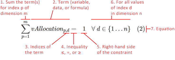
Referring to the numbered annotations:

Many equations involve summing terms (data, variables, or formulae). The symbol for summation is the Greek letter \(\sum\) (sigma). We put symbols below and above the sigma to specify which dimension we're summing and the specific values in that dimension. In this case, we're summing the \(m\) dimension from 1 to \(p\).
The equation will include one or more terms. In this case we're summing the \(vAllocation_{p,d}\) variables.
The \(vAllocation_{p,d}\) variables are using two indices, \(p\) (people) and \(d\) (desks). We're summing over all values of the \(m\) dimension.
An equation will generally include an inequality, i.e. \(\le\), \(=\), or \(\ge\). All parts of the equation to the left of the inequality are referred to as the left-hand side (LHS), and all parts to the right are referred to as the right-hand side (RHS).
The RHS of the equation may be a number, as in this example, or a collection of terms (possibly also including summations).
We must specify what to do with each dimension. In this example, we have only one term, where the \(m\) dimension is summed. The final part of the equation specifies what to do with the \(n\) dimension — that is, make a copy of the constraint for all (\(\forall\)) values of the \(n\) dimension with index values in (\(\in\)) the range 1 to \(n\). Some formulations use equivalent notation like \(\forall d \in N\) where \(N\) represents a set defined as \(N = \{1..n\}\).
Equations are often numbered, using notation like (2), so that they can easily be referred to.

This is just a sample of the mathematical notation that can be used in model formulations. For a more comprehensive list of notation, see: Math symbols list.

Interpretation of the formulation

Given this notation, each equation in the formulation is interpreted as follows:

Equation (1), Objective function. Calculates the total \(dPreference_{p,d}\) across all people and all desks, given the desk \(vAllocation_{p,d}\) decision for each person. Equations like this are often implemented in an Excel formula using the SUMPRODUCT function (as we do in the example spreadsheet).
Equation (2), Constraint. For each person \(p\), sum the \(vAllocation_{p,d}\) variables and set the result equal to 1. Do this sum for each desk \(d\). This produces \(n\) constraints, which together say that each desk is allocated to exactly one person.
Equation (3), Constraint. For each desk \(d\), sum the \(vAllocation_{p,d}\) variables and set the result equal to 1. Do this sum for each person \(p\). This produces \(m\) constraints, which together say that each person is allocated exactly one desk.
Equation (4), Constraint. The \(vAllocation_{p,d}\) of a desk \(d\) to a person \(p\) can occur only if the \(dAvailability_{p,d}\) of that desk to that person is non-zero, for all desks and for all people.
Equation (5), Variable. The \(vAllocation_{p,d}\) of a desk \(d\) to a person \(p\) is a binary decision, where 1 means that an allocation occurs, otherwise an allocation does not occur.
Equation (6), Data. The \(dAvailability_{p,d}\) of a desk is defined such that 1 indicates desk \(d\) is available to person \(p\), otherwise it is unavailable.
Equation (7), Data. The \(dPreference_{p,d}\) of person \(p\) for desk \(d\) is a number, where a higher number indicates a greater preference (because we're maximizing the sum of the chosen preferences). The ordering of the numbers matters, but the size of the numbers is arbitrary.
Equation (8), (9), Indices. Person \(p\) and Desk \(d\).
Equation (10), (11), Dimensions. The number of People \(m\), and number of Desks \(n\).

Note that we assume that the number of people equals the number of desks — that is, \(m = n\). If that is not the situation, then we would need to modify the constraints slightly.

Implementation

Figure 3. Desk preferences for each person

Specify the data

Our model formulation is defined over two dimensions — people and desks. This fits nicely with the two-dimensional grid structure of a spreadsheet.

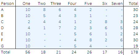
Figure 3 shows the desk preference data for each person. For example, Person C has expressed their highest preference (8) for Desk Six, and their lowest preference (1) for Desk Four. It seems that Desk One is especially popular, including amongst people who are not able to sit there (refer to the Availability table).

There are similar tables for the availability data, allocation variables, and a calculation of the allocated preferences.

Solver model

We use range names to mirror the formulation

Since we're building our model in Excel, we use range names for many of the model components, where the names mirror those used in the mathematical formulation. The Solver dialog displays those range names, which makes the model easier to understand. Note that we may also give specific components of the formulation their own range names — for example, the LHS components of Equations (2) and (3) have their own names.

Note that the indices that are explicit in the formulation are implicit in the grid structure of the spreadsheet. For example, in Figure 3, rows represent the \(m\) dimension and columns represent the \(n\) dimension. Therefore, the named range dPreference is a two-dimensional block of data.

Objective function

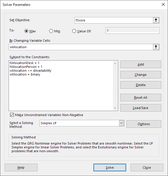
The Solver model is shown in Figure 4. Our objective is to minimize fScore Equation (1), the total of people's preferences given the desk that they are allocated to.

Variables

The model has just one set of variables:

vAllocation. A variable for each person, indicating which desk they are allocated to.

Constraints

The constraints are:

fAllocationDesk = 1 Equation (2). Each desk is allocated to exactly one person. The summation is done in the formula.
fAllocationPerson = 1 Equation (3). Each person is allocated to exactly one desk. The summation is done in the formula.
vAllocation <= dAvailability Equation (4). An allocation can occur only if that combination of desk and person is available.
vAllocation = binary Equation (5). The vAllocation variables are binary.

Solution method

This is a pure Integer Program (IP), using binary variables, so it can be solved efficiently using the Branch and Bound version of the Simplex method. The model is small, so it can be solved using either Solver or OpenSolver. An optimal solution is found in less than a second.

Analysis

Optimal solution

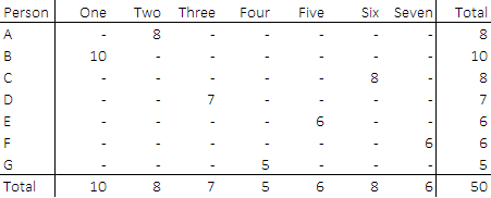
The optimal solution is shown in Figure 5. Key points to note:

Each desk is allocated to one person, and each person is allocation to one desk. Both conditions, as specified in Equations (2) and (3), are necessary.
Some people (for example, Person G) indicated a high preference for a desk that is not available to them (Desk One). The model did not use that preference because such an allocation is prevented by Equation (4).
It is not possible for everyone to be allocated their highest individual preference. Therefore, the model has selected a combination of allocations that maximizes the overall total preference — as specified by Equation (1).

Conclusion

This article shows an example of interpreting a mathematical formulation in the style typically seen in the modelling literature.

Implementing the formulation in an academic paper is often a difficult process. A key place to start is understanding what the mathematical notation means. All going well, that understanding provides a sound basis for building a working model in Excel.

If you would like to know more about this model, or you want help with your own models, then please contact us.

References

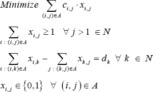
The formulation shown in the title image is for an open tour of the Travelling Salesman Problem, from page 97 of:

Rasmussen, R. (2011). "TSP in spreadsheets: A guided tour". International Review of Economics Education, Volume 10, Issue 1, Pages 94-116.

On the shoulders of giants