Solver Max - Job sequencing to minimize completion time

1 March 2021

"Job sequencing" is a common management problem, especially in manufacturing and production businesses.

That is, given a set of jobs, what is the job sequence that takes the minimum total time?

The benefits from improved sequencing can be substantial, while a poor sequencing solution can be expensive. To illustrate how an optimization model can help us make the decision, in this article we solve a simple job sequencing problem using Solver.

Download the models

The model is available on GitHub.

Situation

We operate a manufacturing business. Our process involves using a single machine to make each of 10 components. Production of the 10 components – known as "jobs" – can be completed in any order. The time required to transition between the jobs depends on the order in which the jobs are completed.

The time taken to do each job, and the time taken to assemble the components, is fixed – so we can ignore those times and just focus on the transition times between jobs.

Our objective is to minimize the time taken to complete the jobs. That is, we want to find the job sequence that has the shortest total transition time.

Model design

Figure 1. Job transition times (minutes)

Potential modelling approaches

There are numerous approaches to modelling job sequencing problems. In this example, we'll utilize an interesting type of constraint available in Solver: the "All Different" constraint.

We want to sequence a set of 10 jobs. We can do that by specifying the position of a job in the sequence as an integer from 1 to 10. Then we define those positions as variables with an All Different constraint. This constraint ensures that we select each position exactly once. We have a calculation of the time to complete the transition from job to job, where we want to minimize the total of those transition times. This approach makes our model very simple.

Define transition times from job to job

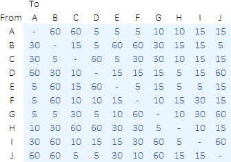
Figure 1 shows a 10x10 matrix of transition times for every combination of two jobs. For example, the transition time from Job A to Job B is 60 minutes, while the transition time from Job B to Job J is 5 minutes. Note that the matrix does not need to be symmetrical – for example, the transition time from Job B to Job A is 30 minutes.

Since our objective is to minimize the total transition time of the job sequence, that's all the data our model needs.

Potential for sub-tours

Our job sequencing model is a type of Traveling Salesman Problem (TSP). That is, we want to "visit" each job only once, in a sequence that minimizes the total transition time. Usually in a TSP we return to the starting point – but that isn't required in this situation, so we have a variant known as the Open TSP.

A common issue with TSP models is the potential for "sub-tours", meaning sequences of steps that are isolated from the rest of the steps. Sub-tours are an undesirable solution, which often require complex model features to avoid. In our situation, sub-tours are not a concern, because the transition time matrix is complete – meaning that there exists a transition from every job to every other job. If it was not possible to do some transitions, then we would need to modify our model to handle potential sub-tours.

Mathematical formulation

Our model's mathematical formulation is shown in Figure 2. That is:

Equation 1. We want to minimize the total transition time to complete all jobs.
Equation 2. The sequence variables are all different.
Equation 3. The sequence variables are integers.
Equation 4. Each job has a transition time to each other job.

Figure 2. Model formulation

\begin{alignat*}{1} &\text{Objective} \\ & \quad \text{Min } fTotalTime \ \ &= &\quad \sum_{k=2}^n \text{dTime}_{i,j} \quad \tag{1} &\begin{array}{l} i: \ vSequence_{i}\ =\ k-1 \\ j: \ vSequence_{j}\ =\ k \end{array} \\ \\ &\text{Subject to} \\ & \quad vSequence_{i} &\ne &\quad vSequence_{j} \quad &\forall \ i \in I, \forall \ j \in J \tag{2}\\ &&&&i \ne j \ \text{(All different)} \\ &\text{Variables} \\ & \quad vSequence_{i} &= &\quad \text{Integer} \quad &\forall \ i \in I \tag{3}\\ \\ &\text{Data} \\ & \quad \text{dTime}_{i,j} &= &\quad \text{Positive real, minutes} \quad &\forall \ i \in I, \forall \ j \in J \tag{4}\\ \\ &\text{Sets} \\ & \quad I, J, K &\ &\quad \text{Job} \tag{5} \\ \\ &\text{Dimensions} \\ & \quad n &\ &\quad \text{Number of jobs} \tag{6} \\ \\ &\text{Bounds} \\ & \quad \text{Non-negative} &\ &\quad \tag{7} \\ \end{alignat*}

Implementation

Define the sequence

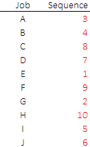
For each of our 10 jobs, we need to define its position in the sequence. This is done via the variables shown in Figure 3. In this example, we have randomly chosen a sequence that does Job E first, then Job G, etc, finishing with Job H in position 10.

Lookup the transition times

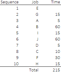
Given a job sequence, we need to get the transition time for each pair of jobs. One way to get the times is shown in Figure 4.

That is:

The sequence steps are specified in order from 1 to 10.
We look up the job assigned each position in the sequence variables (Figure 3) using an INDEX MATCH formula. For example, sequence step 1 is Job E, then Job G, etc, down to Job H as sequence step 10.
Then we need to get the transition time for each pair of jobs in the sequence. To do that we use an INDEX MATCH MATCH formula that looks at the transition times matrix shown in Figure 1. For example, the transition time between steps 1 and 2 in the sequence, which is between Jobs E and G, is 15 minutes. From Job G to Job A is 5 minutes. The last step in the sequence, from Job F to Job H, takes 15 minutes.
Finally, we sum the transitions times, to get the total transition time required to complete the sequence. This value will be our objective function. In this random example sequence, the total transition time is 215 minutes.

Using INDEX and MATCH functions in our calculations makes our model non-linear. Usually non-linear functions should be avoided, as Solver often struggles with non-linear models, especially those that use discrete functions. Instead, we prefer to build linear models because they are easier to solve and are (in theory) guaranteed to find an optimal solution.

We could reformulate our model to be linear, but that would make it significantly more complex. However, in this situation our model is simple, and we want to illustrate a way to handle non-linear models like this.

Solver model

Objective function

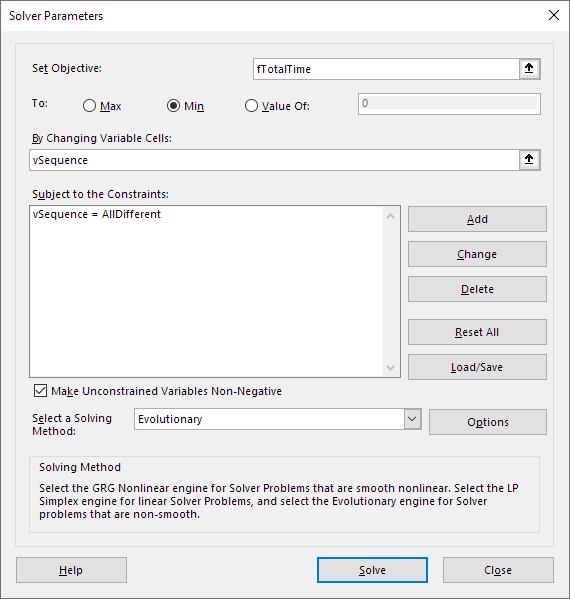
The Solver model is shown in Figure 5. Our objective is to minimize fTotalTime, as described above.

Variables

The model has only a single set of variables:

vSequence. This is the position of a job in the sequence, as shown in Figure 3.

Constraints

There is only one constraint:

vSequence = AllDifferent. This type of constraint is created using the dif relationship. An All Different constraint requires each of the sequence variables to be a unique integer from 1 to 10 (since there are 10 variables).

Solver has an All Different constraint type built-in. Such constraints can also be formulated for OpenSolver, though that is more complex.

Solution method

Due to our use of INDEX and MATCH functions, this model is non-linear. The Evolutionary method can be a good choice for this type of model, so we'll use that.

Though note that the Evolutionary method has significant drawbacks, including:

Even though our model is small, with only 10 variables and 1 constraint, Solver typically takes 10s of seconds to find a good solution. This is quite slow for a model of this size.
There is no guarantee that Solver will find an optimal solution when using the Evolutionary method. More generally, the Evolutionary method may fail to find any solution. Restarting Solver with different initial variable values, or solving the model two or three times in succession, may increase the probability of finding a solution.

Analysis

Optimal solution

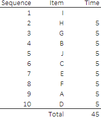
Given our data and model, Solver's solution is shown in Figure 6. We ran Solver a few times, with most solutions have a total transition time of 50 or 55 minutes. The best solution Solver found has a transition time of 5 minutes for each job, for a total transition time of 45 minutes.

Compared with our initial, random solution of 215 minutes, this solution of 45 minutes is a reduction of 79% – a substantial improvement. Looking at the transition time matrix, it isn't obvious that such a good solution is possible.

Since we're using the Evolutionary method to solve our model, we generally don't know how good the solution is. However, in this case, we can deduce that a total transition time of 45 is an optimal solution because each of the transition times is the shortest possible.

Distribution of all solutions

The large difference between our random solution and Solver's optimal solution raises an interesting question: What is the range of possible solutions for this problem?

Many problems have such as enormous solution space that it is not possible to answer that question. However, the number of possible solutions for this problem is relatively small. That is, for a sequence of 10 jobs, there are 10! = 3,628,800 possible solutions. This is sufficiently small that we can explore the solution space by using VBA to enumerate all possible solutions and then plot the distribution of total transitions times, as shown in Figure 7.

Figure 7. Distribution of total transition time for all possible solutions

Key points to note about the total transition time distribution:

The best solution has a total transition time of 45 minutes, as found by Solver above.
A total transition time of 45 occurs twice. The two alternative optimal sequences are: I, H, G, B, J, C, E, F, A, D and F, A, D, H, G, B, J, C, E, I.
Our random sequence, shown in Figures 3 and 4, has a total transition time of 215 minutes, which is close to the middle of the distribution.
Good solutions are exceedingly rare. Only 0.012% of the solutions (446 out of 3,628,800) have a total transition time of <= 60 minutes. The best 1% of solutions have a total transition time of less than 100 minutes.
The Evolutionary method is an excellent approach to solving this model, as it always finds a solution within the top 0.012% of all possible solutions. Such good performance isn't always true, but it works well for this model.
The worst solution is 495 minutes, which occurs 8 times.
With up to 60 minutes per transition, we potentially could have had a worst solution of 9 * 60 minutes = 540 minutes. However, that situation doesn't occur in this example data.

Limitations of enumeration

It is feasible to enumerate all solutions in this example, as 10 jobs has a total of only 3.6 million solutions. Since enumeration is possible, we don't need an optimization model to solve this problem.

However, as the problem size increases it soon becomes impossible to enumerate all solutions. For example, if we double the number of jobs to 20, then there would be 20! = 2.4 million million million possible solutions. This is obviously too many to enumerate.

To illustrate the magnitude of that number, our VBA procedure took 81 minutes to enumerate the 3.6 million solutions for 10 jobs. At that rate it would take around 100 million years for VBA to enumerate all solutions for 20 jobs.

Conversely, we could expand our model to find a good sequence for 20 jobs. Solver copes with 20 jobs without any significant issue. It quickly finds a good solution – though, since we can't enumerate all possible solutions, it is unknown if that solution is optimal.

The fact that we can solve even that expanded model in a reasonable time illustrates the power of this type of modelling.

Conclusion

This model is a simple, though powerful, example of solving a job sequencing problem in Excel. Our model also demonstrates that, in the right circumstances, the Evolutionary method can be a useful way to solve specific types of problems.

If you would like to know more about this model, or you want help with your own models, then please contact us.

Excel
Solver

Job sequencing to minimize completion time