13 December 2023

We conclude our article series looking at a common modelling issue: The solution is optimal, but not practical.
In a previous article of this series, we solved Model 3 to optimality with the full data set of 100 items. Given the large memory requirements of Model 3, a data set with 100 items is close to the maximum that we can solve on our modelling computer. But what if we need to solve a larger data set?
Model 4 provides one approach, using a heuristic random column generation technique that finds very good solutions, though they are not guaranteed to be globally optimal.
The variants of Model 5 all have even more variables and constraints than Model 3, so they don't help us solve larger data sets.
To find guaranteed, globally optimal solutions we need to use Model 3. That requires a computer with more memory – potentially a lot more memory. We could upgrade our modelling computer. If there's a need to often solve very large models, then that would likely be the best option. But if the need is less frequent, then a potentially cost-effective solution is to use a virtual machine in "the cloud".
In this article, we adopt the latter approach. We describe, in detail, setting up a Google Compute Engine, provisioned with 128 GB RAM, and using it to solve Model 3 to global optimality with a data set that is larger than we can solve on our local computer.
Articles in this series
The articles in this "Optimal but not practical" series are:
- First attempt. Model 1: Non-linear model that finds optimal solutions for small data sets, but not for the full data set.
- Linear, partial data set. Model 2: Linearized model using a small sub-set of the full data. Finds local optima.
- Full data set. Model 3: Extends Model 2 to use the full data set. Finds globally optimal solutions, but requires a large amount of memory.
- Column generation. Model 4: Variation of Model 2, with randomly-generated columns. May find globally optimal solutions, though not guaranteed to do so.
- Either/or BigM. Model 5a and 5b: Explicitly models rotation of the items using BigM constraints. Three times larger than Model 3, so difficult to solve.
- Either/or Disjunction. Model 5c: Explicitly models rotation of the items using Pyomo's Generalized Disjunctive Programming (GDP) extension.
- Virtual machine. We set up a Google Compute Engine with 128 GB of RAM to run Model 3 on data sets larger than we can run on our local modelling computer.
Download the model
The models described in this series of articles are built in Python using the Pyomo library.
The files are available on GitHub.
Situation
The situation is the same as for the previous models in this series.
Resource requirements for Model 3
Before we set up a virtual machine, let's look at the resource requirements for Model 3, given a variety of data set sizes and using the HiGHS solver.
Figure 1 shows the observed number of variables, memory usage, and run time for Model 3 on our local modelling computer as we increase the number of items from 20 to 110:
- Number of variables. In this model, the number of variables is \(i^3 + i^2\), where \(i\) is the number of items. A data set with 100 items requires 1,010,000 variables, while we can extrapolate that a model with 200 items would require 8,040,000 variables.
- Memory usage. The model's peak memory usage increases in a fairly smooth way, with a cubic function being a good fit. 100 items use 5.5 GB of RAM. Our modelling PC has 16 GB of RAM. We solved a data set of 115 items but, allowing for the operating system and other applications, we ran out of RAM when attempting to solve larger data sets. Extrapolating the fitted function suggests that we would need about 40 GB of RAM (plus operating system, etc.) to solve a data set with 200 items.
- Run time. A cubic function is also a good fit for the run time observations. A data set with 100 items takes 434 seconds. Extrapolating to 200 items suggests a run time of about 2.5 hours.
Of course, our extrapolations for memory usage and run time potentially have a large margin of error. Even so, it looks like a 200-item data set can be solved in a reasonable time, provided we have more RAM.
Cloud computing
Rather than buying a computer with more memory, we decided to try using a cloud computing service to solve the model. Cloud computing services have become popular in recent years, for many different purposes. For our purpose, all we need is access to more memory.
There are several competing cloud computing services available, some of which focus on optimization modelling. The most commonly used dedicated service is NEOS Server. We've used NEOS previously, for example in the articles We need more power: NEOS Server and Taking a dip in the MIP solution pool. However, NEOS has a limit of 3 GB of RAM, which is much too small for our Model 3 with 200 items.

We haven't conducted a comparison between the various cloud services that are available. For this experiment, we chose to use the Google Cloud service simply because it is a convenient, general-purpose service. Google also offers a free trial, with a US$300 credit that is valid for 3 months. Other services may be cheaper and/or have better features for specific applications, but that is an analysis for another time.
So, we set up a Google Cloud account with the objective of solving an optimization model that is larger than we're able to solve on our local machine. The following sections document the process we used to set up and run the model. If you have a similar issue, then perhaps this article will be useful to you.
Setting up a Virtual Machine
Choosing a Compute Engine option
Google offer a wide range of cloud computing services. Each service has a specific set of fees, which can be estimated using the Google Cloud Pricing Calculator.
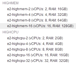
We want a general-purpose virtual machine, which Google call a "Compute Engine". A Compute Engine can be configured in many ways, from 2 CPUs and 4 gigabytes (GB) of RAM, up to hundreds of CPUs and terabytes (TB) of RAM.
The HiGHS solver typically uses only one or two CPUs, so the number of CPUs isn't important in our case. We estimate that a data set with 200 items needs 40 GB of RAM plus operating system, etc., so 64 GB of RAM might be enough. But we should allow some headroom in case the solver needs more. Therefore, we select a Compute Engine, from the E2 series, with 16 virtual CPUs and 128 GB of RAM, as shown in Figure 2.
Google's cloud pricing calculator estimates that our chosen Compute Engine option will have a fixed cost of US$1.00 per month for the minimum 10 GB of disk storage (for the operating system, our files, and any applications we install), plus a usage rate of US$0.73/hour (incurred only when the virtual machine in on). Assuming usage of 40 hours per month, the estimated cost is about US$30 per month. Note that the fees vary by location, and they change over time.
Create a Project and start the Compute Engine
We already have a Google account, so we log into Google Cloud using that account. The first thing we need to do is create a Project. The process is described in the documentation at Create Project.
Within the project's dashboard, we can assign resources. So, we select our chosen Compute Engine option and, a moment later, it is ready to go.
Having selected a Compute Engine, we open its administration webpage within Google Cloud. The administration webpage provides many tools for managing the Compute Engine instance. To start the Compute Engine, click the START/RESUME button. When starting the Compute Engine, we're reminded that it will incur fees while running.
After starting the Compute Engine, the standard way that Google provide to make a secure connection to it is to open a command line terminal using the SSH-in-Browser application. This is done by selecting the SSH button on the Details tab. After establishing a secure connection, the SSH-in-browser application looks like Figure 3.
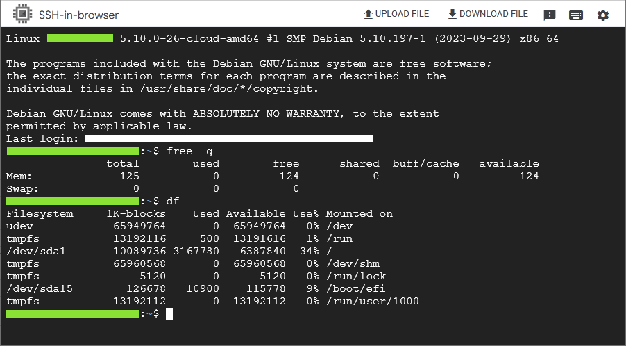
Our specific instance is running Debian Linux (we could have chosen Windows, though that option incurs an additional fee). Using the commands free -g and df, we see that we have 125 GB of RAM available (presumedly the 128 GB we selected, less some overhead), along with a useful amount of disk space (after installing Python, some libraries, and our model files). Note that we've obscured some details, such as our username and the name of this instance.
Install Python
The Compute Engine is bare bones. We want to run some models written in Python, so we need to install Python and the libraries that we want to use.
A useful blog article, Schedule Python scripts on Google Cloud Platform from scratch, describes setting up a Compute Engine and installing Python. We follow their advice for updating the existing operating system and installing Python in a virtual environment (like the setup we have on our local computers, described in Set up a Python modelling environment). That is, we run the following commands (one at a time) in the Compute Engine's command line interface:
sudo apt update
sudo apt install python3 python3-dev python3-venv
sudo apt-get install wget
wget https://bootstrap.pypa.io/get-pip.py
sudo python3 get-pip.py
python3 -m venv env
Google provide an article that also describes setting up Python in a Compute Engine, Getting started with Python on Compute Engine. After ensuring that we've done the "Before you begin" steps, the key thing we need to do is install the libraries that we want to use. Therefore, we create a text file, called requirements.txt, that lists the libraries we want:
pyomo
highspy
pandas
numpy
openpyxl
psutil
Specifically, we want to use Pyomo and the HiGHS solver, along with some utilities. This list matches the libraries that we include in Model 3, except for json and os, which are standard in Linux, so we don't need to include them.
To install the listed libraries, we run the following in the SSH-in-browser's command line interface:
pip3 install -r requirements.txt --user
We're not going to run a HTTP server in our Compute Engine, so we don't need to follow the other commands in Google's article.
Running our Python model in the Compute Engine
To run our Python model in the Compute Engine, we need to upload the model and data files. Rather than using a Jupyter Notebook, we put the code for Model 3 into a single Python plain text file. We also make some minor changes along the way to suit the new environment, like using print rather than display for the results.
The SSH-in-browser application conveniently includes a button for uploading files. Using that button, we uploaded the code and data files to our Compute Engine. Even though we're using a Linux operating system, the data in Excel files works OK.
We can edit the code using the built-in vi text editor, which is basic but sufficient for making minor changes to the code, though not as convenient as the NotePad++ text editor that we normally use on Windows. For example, Figure 4 shows vi in INSERT mode for editing the data file name.
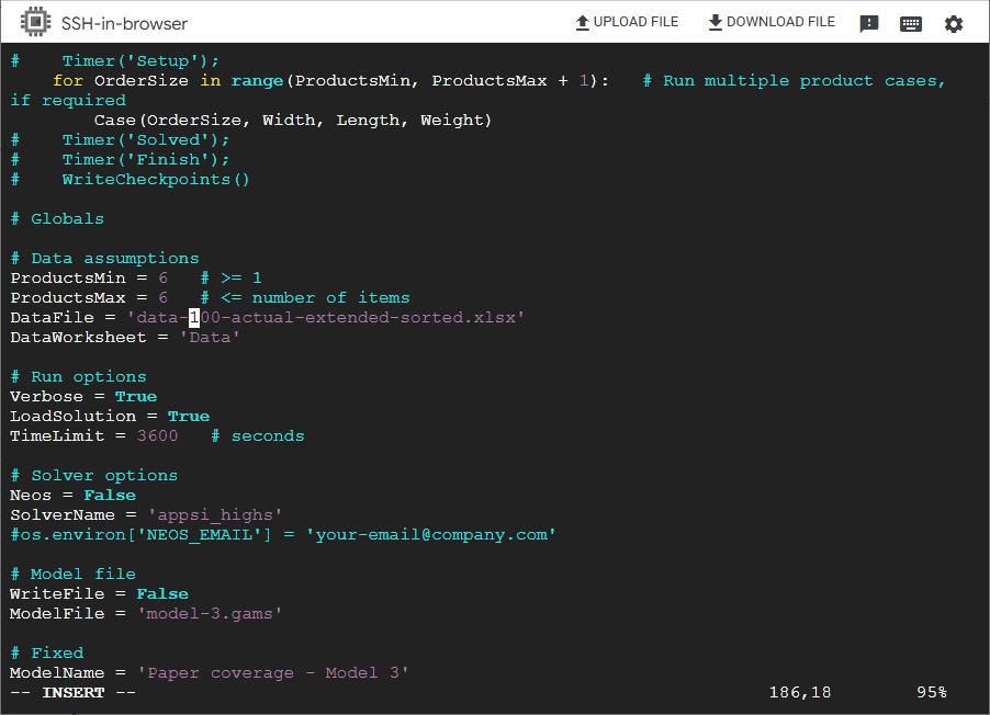
While vi works, we generally edited files on the local computer and then transferred them to the Compute Engine. This is easier, and has the added advantage of having a local copy of the files.
Running the code simply requires using the command line to call Python with the model file (noting that we installed Python using the name python3):
python3 model-3.py
To test that the Compute Engine setup works, we ran the sample data with 20 items. It solves in a fraction of a second, returning the optimal solution.
All good so far. The Compute Engine works, and we can use it to solve a Python model using the HiGHS solver. But then we ran into a problem.
Compute Engine disconnects every 10 minutes
Our model runs correctly using a small data set. But if we run a larger data set, then the solver's progress is lost because the SSH-in-browser application disconnects after 10 minutes. That is, when the HiGHS solver is working on the model, SSH-in-browser treats the connection as idle, so it disconnects. Presumedly, it disconnects to prevent incurring unnecessary fees when the Compute Engine isn't being used – but our Compute Engine is being used, it just doesn't generate any network traffic.
This issue is discussed in the Google Cloud documentation, in the troubleshooting section Idle Connections. Although the issue is discussed, Google unhelpfully does not provide a solution for the SSH-in-browser application. We searched for a way to keep the connection active in our circumstance using the HiGHS solver in the SSH-in-browser application, but we were unsuccessful.
PuTTY
An alternative to the SSH-in-browser application provided by Google is to install and use the PuTTY application for Windows. Getting PuTTY to work with Google Cloud requires a few steps, as follows.
First, we install PuTTY on our local machine. Then, to connect to the virtual machine, we need to generate SSH keys. The Compute Engine already includes SSH keys that it generated automatically to enable us to connect using SSH-in-browser. But we need additional keys for PuTTY.
A separate application, PuTTY Key Generator, is used to generate a pair of SSH keys – one public key and one private key. So, start the PuTTY Key Generator application and click the Generate button. The process, after clicking the Generate button, but before the keys are created, is shown Figure 5. You need to move the mouse over the blank area, to add randomness to the process.
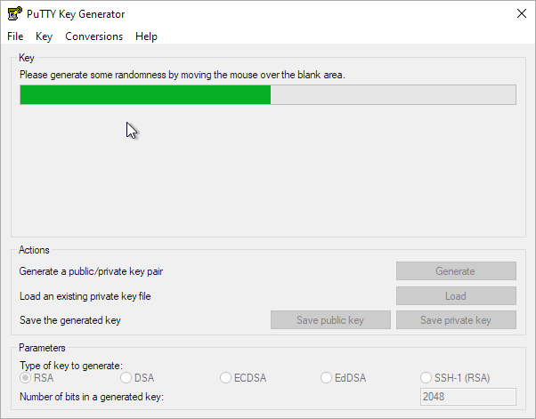
It is recommended that you protect the private key using a "Key passphrase" that you enter in the dialog once the keys are generated. Note the passphrase, as you need it each time you connect to the Compute Engine using PuTTY. Then save the private key to a file in a secure location. Keep the Key Generator application open. For more description of the process see Using PuTTYgen on Windows to generate SSH key pairs.
Back in the Compute Engine's administration webpage, select the DETAILS tab and click the EDIT button. Amongst the many options is a facility to add a new SSH public key. Add a new key and copy/paste the public key from the PuTTY Key Generator (which can then be closed). Save the edits.
Start the PuTTY application. To connect to the Compute Engine, we need to do three things: enter the Compute Engine's external IP address, ask PuTTY to keep alive the connection, and include the private key file.
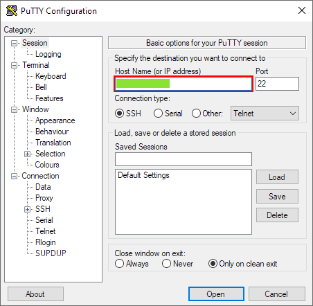
The Compute Engine's External IP Address is shown in the Network Interfaces section of the Compute Engine's DETAILS tab. We sometimes need to refresh the webpage before the address is updated, otherwise it just says "Ephemeral" (meaning that the IP Address may change each time the Compute Engine is started). Copy the External IP Address and paste it into the Session category's Host Name (or IP address) field in PuTTy, as shown in Figure 6. Port 22 and the other values are OK.
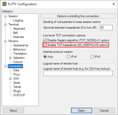
At the top level of PuTTy's Connection category is an option called "Enable TCP keepalives (SO_KEEPALIVE option)", which needs to be selected, as shown in Figure 7. This will keep PuTTY from disconnecting every 10 minutes, enabling the solver to run for as long as it needs.
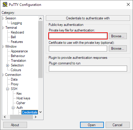
Also in PuTTy's Connection category, under the SSH > Auth > Credentials section, browse to and select the private key file saved earlier, as highlighted in Figure 8.
All the other options are left as their defaults. You can save the configuration, though the IP address will need to be updated each time.
Click the Open button to start the secure connection. As shown in Figure 9, in the "login as" field, enter the Username listed in the Compute Engine's administration page next to the SSH key you added. PuTTy will automatically access the public key. When asked, you also need to enter the passphrase that you created earlier.
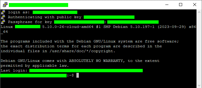
We now have a command line interface to the Compute Engine, much like we had with the SSH-in-browser application. The key difference is that this connection stays active beyond 10 minutes.
Caution: KEEPALIVE incurs fees
There's a reason why the default connection method, via SSH-in-browser, disconnects after being idle for 10 minutes. That is, Google Cloud charges fees for resource usage. If the Compute Engine is active, then it will incur fees.
Selecting the KEEPALIVE option solves the problem of the connection closing after 10 minutes while the solver is running. But keeping the connection alive uses Compute Engine resources and so incurs fees. Therefore, you need to manually close the PuTTY session and STOP the Compute Engine (via its dashboard) when the Compute Engine is not being used, otherwise you will incur fees.
Transfer files using WinSCP
The SSH-in-browser application includes buttons for uploading and downloading files. The PuTTy application doesn't have those options. In any case, the WinSCP application is a better tool for transferring files between the VM and a local machine.
So, assuming you're using Windows, download WinSCp and install on the local machine. If not, then install some other similar software.
Connecting to the compute engine using WinSCP is similar to using PuTTY. That is, we need to specify the Compute Engine's IP address, enter our user name, set the keep alive option, and specify the private key file. These steps, some of which are under the Advanced drop-down menu, are shown in the following figures.
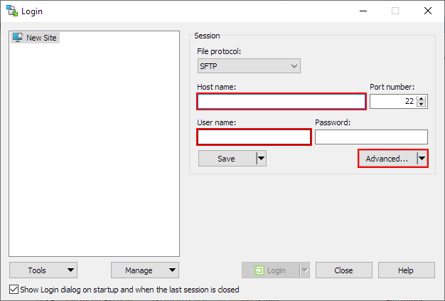
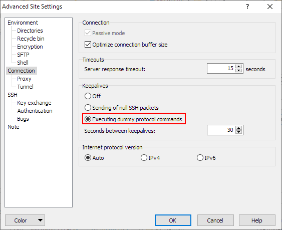
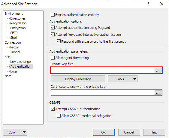
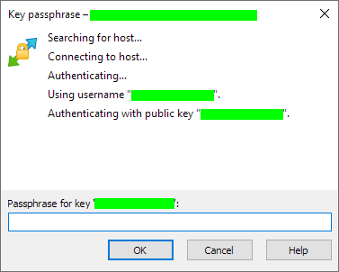
Having completed the setup, return to the WinSCP login dialog and click the Login button. A dialog shows the connection steps and, all going well, asks for the key passphrase that we created earlier. Enter the passphrase and click the OK button, as shown in Figure 13.
Once connected, WinSCP shows the local and Compute Engine folders side-by-side, like the screenshot from WinSCP’s documentation shown in Figure 14.
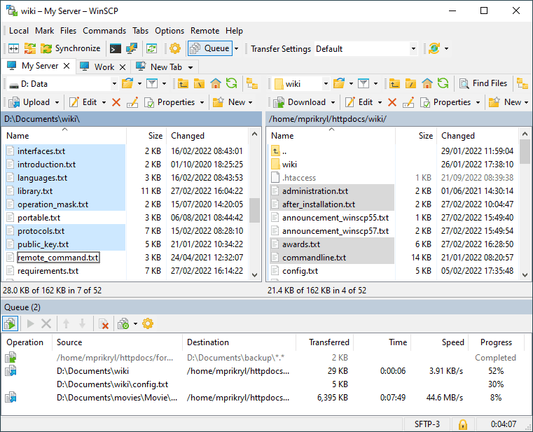
In WinSCP you can create folders, drag-and-drop files between the left (local) and right (Compute Engine) panels, etc.
Solve Model 3 with a large data set
Finally, we're ready to solve Model 3 using a large data set – which is the point of setting up the Compute Engine.
Running the model is the same as previously, except that we're using PuTTY and WinSCP to connect to the Compute Engine. The difference is that the connection remains active, rather than disconnecting after 10 minutes.
With 200 items, our model has over 8 million binary variables. Extrapolating from smaller data sets, we expect the peak memory usage to be around 40 GB, and the solve time to be about 2.5 hours. However, there is significant uncertainty about these estimates, further compounded by running the model in a different environment.
The actual number of variables, memory usage, and run time are shown in Figure 15. The orange dots are for the local machine and the green dots are the Compute Engine. The number of variables is the same on both machines. We also ran some smaller cases on the Compute Engine, for comparison.
It turns out that the Compute Engine takes almost 3 hours to solve Model 3 with a data set of 200 items. This is longer than our extrapolated estimate, though not by much. Importantly, it does solve to optimality. This is an improvement over our attempts on the local machine.
For the 200-item case, the peak memory usage reported by Python is just over 40 GB – very close to our estimate. The Compute Engine dashboard recorded peak memory usage at 56 GB, including the operating system and other processes. So, a 64 GB Compute Engine would have been sufficient – though only just. Therefore, we didn't need to pay extra for 128 GB of RAM.
Solution with 200 items
The solution found by the HiGHS solver for 200 items using Model 3 is the same as the best solution we found earlier using Model 4 with a sub-set of the candidates. Model 4 isn't guaranteed to find globally optimal solutions, so it is reassuring that Model 4 performs well with a larger data set.
Assessment of using cloud computing for optimization modelling
Cost-effectiveness of using a Compute Engine
Our Compute Engine costs US$0.73/hour while it is on. With a run time of almost 3 hours, solving the 200-item case on the Compute Engine costs about US$2.25, including some time for us to set up the run and retrieve the results. This is excellent value, provided the Compute Engine doesn't need to be used often.
But we do need to be careful not to incur unexpected fees. For example, while we were experimenting with the Compute Engine, we accidentally left it on overnight after it had finished solving a model. That mistake cost about US$8.00. Without diligent management of the Compute Engine service, it would be easy to incur significant fees. Google offer budget alerts and limits to help avoid that situation – it would be wise to setup alerts and limits, to ensure you don't get unexpected fees.
Even larger data sets?
Having solved Model 3 with 200 items, we could attempt even larger data sets. For example, a data set with 1,000 items would require 4 to 5 terabytes of RAM. That might be possible using a Compute Engine.
Google's cloud calculator indicates a cost of around US$20,000 for a "m2-ultramem, vCPUs: 416, RAM: 5888 GB" Compute Engine running for the 3 to 4 weeks we estimate it would require to solve a model of that size. Such a cost is unlikely to be worthwhile, firstly because there's no guarantee that the model would solve successfully and, secondly, because we can already solve a model of that size using Model 4 – albeit finding good, though not necessarily globally optimal, solutions.
Another advantage: Flexible configuration
Finally, another advantage of using a virtual machine is that the configuration is flexible.
For example, after completing the paper coverage modelling described above, we used the Compute Engine service for a different project. In that case, we didn't need so much RAM, but speed was more important. So, we simply edited the Compute Engine's configuration to have 4 faster CPUs and 32 GB RAM. Since RAM is an especially expensive resource, the cost of that configuration was just over half that of the configuration we had been using.
In addition, we can make multiple connections to the Compute Engine simultaneously. The paper coverage model uses a lot of RAM, so we could run only one instance at a time. The other project's model uses much less RAM, but we wanted to run it many times with different input data each time. Since the HiGHS solver mostly uses only one CPU, occasionally two, we opened three PuTTY instances, each connected to the same Compute Engine. Then we ran three instances of the model simultaneously, using between 75% and 100% of the Compute Engine's CPU capacity.
We could have chosen a configuration with more CPUs, to run even more instances in parallel, though that would take a bit more effort to manage.
Overall assessment
Our experience of using a Compute Engine to solve an optimization model was mostly positive.
Having the default application disconnect every 10 minutes was a hassle. It took some time to find a work-around, though the combination of PuTTY and WinSCP is better than the default SSH-in-browser application.
Cost managment is a concern. It would be easy to incur significant, unexpected fees if the cloud computing service is not managed carefully. Nonetheless, with close monitoring, using a virtual machine can be a cost-effective way to gain access to computing resources that are not be available locally. The flexible configuration of a virtual machine is also useful.
Using a dedicated optimization service, like NEOS Server, requires less setup and management, and it has the advantage of having access to a wide range of solvers. But if you need more control over the available resources, then cloud computing is a viable and cost-effective tool.
Conclusion
In this article, we describe setting up a Google Compute Engine virtual machine in the cloud and using it to solve Model 3 to global optimality. Using the Compute Engine, we're able to solve a data set that's much larger than we can solve on our local computer, because of Model 3's large memory requirements.
A virtual machine is a potentially cost-effective and flexible way to gain access to computing resources that are not available locally. Provided, that is, those resources are needed only occassionally. If greater computing resources are need often, then it is likely to be better to invest in local resources. The Compute Engine also needs to be carefully managed, to avoid incurring unexpected expenses.
This article concludes our "paper coverage" modelling series.
If you would like to know more about this model, or you want help with your own models, then please contact us.
References
This series of articles addresses a question asked on Reddit:
Require improved & optimized solution, 14 September 2023.
