9 July 2021

There are many tools for implementing and solving optimization models. At Solver Max we specialize in using Solver/OpenSolver in Excel and in the Python programming language, using a library such as Pyomo, CVXPY, or PuLP.
Each tool has advantages and disadvantages, including:
- Excel is, by far, the most widely-used analysis tool. It provides a visual environment for building models, with many built-in tools for analyzing and visualizing data. Excel is relatively easy to get started with, so many people are familiar with using Excel for modelling, analysis, and presentation of results. Prototyping a model in Excel is generally easier than in Python. Excel also has great depth – much more than most people realize. While Excel's grid structure makes data easy to see, its rigidity can complicate the handling of data that varies in size. Consequently, Excel models may not be as flexible as those created using a programming language.
- Python is a popular programming language. Libraries like Pyomo, CVXPY and PuLP handle much of the complexity of the optimization process (like the Solver and OpenSolver add-ins do in Excel). But learning how to program in Python can involve a steep learning curve, which is quite a barrier to entry. Consequently, far fewer people are familiar with programming in Python. Even if the optimization model developer is comfortable with Python, many model users may prefer a more familiar environment for interacting with a model.
To compare Excel and Python, we replicate a Python optimization model described in the blog How to schedule flights in Python. The source article describes the Python implementation. Here we focus on an equivalent Excel implementation. Towards the end of this article we provide a brief comparison of the two implementations.
Download the model
The models are available on GitHub.
Situation

We own an airline that needs to schedule aircraft to cover all upcoming flights.
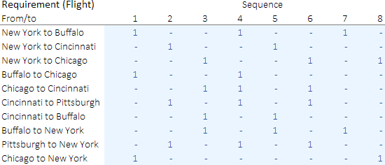
As shown in Figure 1, there are 10 flights between 5 cities (New York, Chicago, Cincinnati, Buffalo, and Pittsburgh), arranged in 8 potential sequences. Each sequence consists of multiple flights, starting and ending in New York. The flights in a sequence are indicated by a 1 in the table.
For example, reading down the column for Sequence 1, the first sequence is from New York to Buffalo, then Buffalo to Chicago, and finally Chicago to New York. Similarly, Sequence 8 is from New York to Chicago, then simply returns from Chicago to New York.
We need to ensure that all 10 flights are covered by selecting some combination of the sequences.
Each sequence has a cost and total hours to complete (over the planning period), as shown in Figure 2. For example, Sequence 1 has a cost of $5,000 and takes a total of 396 hours over the planning period.

Our objective is to minimize the total cost (in units of $1,000) of the flight schedule, while ensuring that each required flight is covered by at least one aircraft. Selecting all sequences would incur a total cost of $43,000 though, of course, we hope to meet the requirements by selecting only a subset of the sequences and hence incur a lower cost.
We may also want to limit the total duration of the selected sequences, so we include an assumption for a cap on the total duration.
Model design
Binary variables to select sequences

We use binary variables to indicate which sequences are selected, as shown in Figure 3. In this solution, sequences 1, 5, and 6 are selected.
Implementation

The model implementation is very simple. Given a selection of sequences, we can calculate the total cost and duration – as shown in Figure 4.
That is, for each characteristic, we calculate the SUMPRODUCT of the selection variables and the corresponding flight data.
Solver model
Objective function
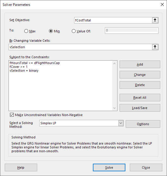
The Solver model is shown in Figure 5. Our objective is to minimize the total cost fCostTotal.

Variables
The model has one set of variables:
vSelection. Binary variables indicating whether to select each flight sequence.
Constraints
The constraints are:
fHoursTotal <= dFlightHoursCap. Cap on the total hours used by the selected sequence.fCover >= 1. Each flight must be covered by at least one sequence.vSelection = binary. The selection variables are required to be Binary.
Solution method
All the model's relationships are linear, so we can use the Simplex method.
This model is sufficiently small that either Solver or OpenSolver can be used.
Analysis
Optimal solution
The source article explores two scenarios, so we do the same:
- Scenario 1. No cap on the total schedule hours. Since the model includes a constraint on the total schedule hours, we simply set the cap to be sufficiently high that the constraint isn't binding. That is, the duration of all sequences is 4,250 hours, so any cap of greater than 4,250 hours will not affect the solution. The model selects flight sequences 1, 2, and 3, with an optimal schedule cost of $13,000 and duration of 1,770 hours.
- Scenario 2. Cap of 1,700 hours. Since the cap is lower than Scenario 1's optimal solution, that solution is no longer feasible. To comply with the cap, the model select flight sequences 1, 5, and 6. Sequences 5 and 6 are more expensive, leading to a total cost of $20,000 and duration of 1,614 hours.
In this example, Solver in Excel finds the same solutions as those found by CVXPY in Python. If there are alternative optima, then there is no guarantee that the different tools would find the same solutions. We sometimes see that occur when solving the same model with Solver and OpenSolver, or even with different versions of Excel. Similarly, calling different solvers from Python may produce different, alternative optima solutions.
Excel vs Python
In this article, we implemented a scheduling problem in Excel and solved it using the bundled Solver add-in. We could also use the free OpenSolver add-in and open source COIN-OR CBC solver.
The source article implemented the model in Python using CVXPY and solved it using the GLPK open source solver. CVXPY also provides a choice of solvers, including the COIN-OR CBC solver.
We obtained identical results, but the implementation details are very different.
In Excel we built the model in a visual, grid-based environment. First, we defined named ranges for the cost data and the selection variables. Then, in the Solver dialog, we defined the objective function by selecting a range named fCostTotal that refers to a cell containing the formula:
=SUMPRODUCT(SequenceCosts,vSelection)
In Python, all aspects of the model are defined in programming code. For example, after reading the data and assigning it to data structures, the cost data and selection variables are defined as:
c = cost.values
y = cp.Variable(len(c), boolean=True)
The objective function is then defined as:
obj = cp.Minimize(c @ y)
Similarly, in Solver, the coverage requirement and the cap on the total duration are specified as the constraints:
fCover >= 1
fHoursTotal <= dFlightHoursCap
We define the constraints in the Solver dialog by selecting the appropriate cells in the Excel grid and choosing the required constraint relationship (<=, =, or >=).
While in Python, the same constraints are defined as:
constraints = [a @ y >= b, h @ y <= 1700]
To solve the model in Excel, we click the Solve button in the Solver dialog.
In Python, we define the model as the combination of the objective function and constraints, as follows:
prob = cp.Problem(obj, constraints)
We then solve the problem using:
prob.solve(solver=cp.GLPK_MI)
In Excel, the solution is shown in the cells used to define the variables and calculations.
In Python, the solution is printed to the console using a command like:
print(y.value), which displays the result as [1. 0. 0. 0. 1. 1. 0. 0.].
Excel has built-in ways to display the model and subsequent analyses, including tables and charts. Displaying the results and analyses in Python requires additional programming.
Conclusion
This model is a simple example of solving a scheduling problem in Excel compared with Python.
The choice of optimization tool depends on the circumstances, including the model's features and the modellers' and users' familiarity with the tools. It is also a matter of personal preference.
Both Excel and Python require programming to build optimization models. Excel uses functional programming in a visual grid to specify the calculations, along with a dialog box interface to a tool that defines the model relationships. Python uses procedural programming code, assisted by libraries that bundle pre-packaged tools. The means differ, but the results are the same.
Each approach has advantages and disadvantages. It is useful to understand a bit about the different tools that are available, so that you can make an informed decision about which approach is best in your situation.
If you would like to know more about this model, or you want help with your own models, then please contact us.
