8 September 2023
Microsoft recently announced a new Excel feature, Python embedded within Excel. This is great news, as it combines our two favourite tools: Excel and Python. Since our focus is on optimization modelling, we immediately wondered if it is possible to use a Python library to solve optimization models directly within Excel. Spoiler alert, it is!
In this article, we experiment with building and solving a linear program in Excel using the Python SciPy library. Specifically, we replicate the Production Mix model that we previously solved using SciPy as part of our Rosetta Stone series of articles that looked at various Python optimization tools.
Download the model
The model is available on GitHub.
Note that the Python in Excel feature is currently in Beta testing. The feature is not yet widely available, so this model may not work for you.
Situation
We want to know if we can build and solve an optimization model in Excel using a Python library. For this purpose, the details of the model aren't important. But if you want to know, our model is a simple production mix linear program, described in detail in our earlier article.
Python model in Excel
Overview of the model
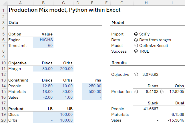
Figure 1 shows our Python linear program model in Excel.
On the left, we have our data in named ranges. On the right, we have Python code in cells that creates the model, solves it, and then reports the results.
We want to maximize profit, but SciPy always does minimization. Therefore, we've made the objective function coefficients negative to mimic maximization.
Enter Python code in a cell
We enter Python code in a cell by either typing a normal formula starting with =py( or use the shortcut CTRL+ALT+SHIFT+P. Either way, the Excel Formula Bar changes to have a green sidebar marked with "PY", indicating that we can enter Python code.
Import libraries
Python in Excel is set up with a selection of more than 400 Python libraries. Unlike a normal Python program, we can use only the libraries that have been made available.
Fortunately, one of the available libraries is SciPy, which is an open-source library that includes many functions for mathematics, science, and engineering. Those functions include a variety of optimization methods.
The first thing we need to do is import the linear programming part of the SciPy library. To do that we enter, in cell H5, the Python code:
from scipy.optimize import linprog
"SciPy"
We make a new line by pressing Enter and enter the code by pressing CTRL+Enter. This cell contains two lines of Python code:
- The first line imports the library. This line must be in a row above the rest of the model as, according to the sparse help within Excel, the Python code runs in "row-major order and then worksheet order".
- The second line is optional. It writes a value to the cell, to provide the user with some information. This is equivalent to
print('SciPy'), except we don't need to use theprintcommand in Excel Python. Without this line, the cell would display "NoneType", which isn't helpful.
Most of the Python cells are marked with an icon at the left of the cell. An exception occurs where we've changed the output to "Excel Value" – which we describe later. If we click the icon, then we can show the Python "card", which provides some information about that cell from a Python perspective.
Get data
Next, we need to get some data from the worksheet named ranges (or we could just use cell addresses) into our Python model. We do this in cell H6, using the xl() function:
Engine = xl("Engine")
TimeLimit = xl("TimeLimit")
ObjCoeff = xl("Margin")
Constraints = xl("Constraints")
rhs = xl("rhs")
VarBounds = xl("VarBounds")
"Data from ranges"
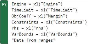
The Python code, as it appears in the FormulaBar, is shown in Figure 2.
This code loads values from worksheet named ranges into Pandas DataFrames. For example, the coefficients for our constraints are in the named range "Constraints", which is cells B14:C16. Therefore, we create a DataFrame called Constraints, with 2 columns and 3 rows, to hold those values.
It isn't necessary to assign the data to the variables Engine, TimeLimit, ObjCoeff, etc. But doing so makes subsequent code easier to read.
Create and solve the model
In H7 we create and solve the linear program model, using the code:
Model = linprog(c = ObjCoeff, A_ub = Constraints, b_ub = rhs, bounds = VarBounds, method = Engine, options = {'time_limit': TimeLimit})
That line sends our data to SciPy's linprog function and assigns the result to the object Model. Specifically:
- The linear program is defined using the matricies
c,A_ub, andb_ub, representing the objective function coefficients, the constraint coefficients, and the constraint right-hand-side coefficients, respectively. Inlinprog, the variables are implicit, so we don't represent the variables explicitly. - We represent bounds on the variables using
bounds. The data for the bounds needs to be transposed relative to the constraint coefficients, though it is not clear why. - Many of the SciPy optimization functions have a variety of methods that can be used. In this case, we specify that the linear program should be solved using the HiGHS solver.
- We can also specify some options for the solve process. In this case, we set a time limit using the HiGHS option
time_limitin seconds. We tested that this works by setting the time limit data, cell B7, to 0. We then got the message "Time limit reached" in the Result, and Success is FALSE.
Since we didn't write any output in this cell, we get the default response from the library: "OptimizeResult".
To check that the model solved OK, in H8 we have the code:
Model.success
That code simply displays a Boolean for the success property of the Model object.
Show results
Having solved our model, we can now get the results.
To retrieve the objective function value, we get the fun property of the Model object. Since linprog always does minimization, but we're maximizing, we need to negate the objective function value. This is, in H12:
-Model.fun
linprog refers to the variables as x, so in H15 and I15 we get their values using:
Model.x[0]
Model.x[1]
The slack values are in the slack property, so in H18 we display them using:
Model.slack
Finally, we get the dual values in I18 using:
Model['ineqlin']['marginals']
Note that the slack and dual values differ from the other results. After entering the code, we right-clicked on the cells and selected Python Output > Excel Value, rather than the default Python Object. This converts the Python value to Excel values – that is, a spilled range showing the DataFrame values. These cells do not have the card icon, even though they contain Python code.
By displaying the Excel Value, we don't have to code each individual element (like we do for the variable values in H15 and I15), and we don't need to know how many elements there are.
Observations and things we learnt along the way
Overall, our experiment is a success
We decided to implement a simple linear program in Excel using Python. This was straightforward, and the resulting code is easy to understand. The model works, and the solution is correct. Therefore, we consider this experiment to be a success.
Python in Excel is very new
One challenge we encountered was that help is hard to find. Documentation for Python in Excel is quite sparse. The feature is very new, so there is little help available online generally. Consequently, working out how to fix issues can be difficult.
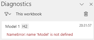
Help within Excel is not always all that helpful. When running the Python code, a Diagnostics pane opens automatically (though it can be turned off), as shown in Figure 3. The Diagnostics pane shows errors messages that, as is the norm for programming languages, are often cryptic.
For example, setting the bounds was tricky. Firstly, we had to work out that the bounds need to be a single range, rather than separate ranges for the lower bounds and the upper bounds. Then we had to work out that the bounds range needed to be transposed relative to how we assumed it should be.
Before we transposed the bounds range, the results cells showed a #PYTHON! error and the Diagnostics pane messages were "TypeError: 'NoneType' object is not subscriptable" and "TypeError: bad operand type for unary -:'NoneType'". It was not obvious, at least to us, that these messages meant that we needed to transpose the bounds data.
Live Python code is useful, but it can be slow
An advantage of using embedded Python code is that our linear program is solved automatically when the worksheet recalculates, rather than having to open a dialog or run VBA code. If we change the data, then we get a new solution automatically, which is great.
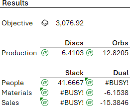
But the Python code is run in the cloud, so updating is quite slow. If we change anything, then each of the Python cards updates one at a time. Expect to often see the #BUSY! value in cells – it is displayed when a call is updating after editing. While cells are waiting to be updated, the icon on the left side of each card cell changes from a black card to a green symbol, like that shown in Figure 4.
In our simple model, it typically takes about 6 seconds to update the 13 cards – and sometimes it takes much longer. Our simple linear program solves almost instantly, so the lag is due almost entirely to communicating with the cloud server where the code is running. For a more complex model, which takes minutes or hours to solve, this lag might become a problem.
Editing code would benefit from a better tool
The Python code is edited in the Excel FormulaBar. While the FormulaBar is OK for editing short Excel formulae, it isn't great for longer code.
Microsoft have released an editor that enables you to "write and edit Python formulas in Excel using a dedicated code editor with similar capabilities as those available in Python notebook environments".
Introducing the Python Editor from Excel Labs
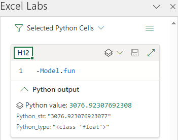
While creating the model, we expanded the FormulaBar to have several lines. Normally that would indicate an excessively long formula. But, when using Python, multiple lines of code in a cell will likely be normal. Conversely, dividing a Python program into one line of code per cell would be unnatural and difficult to work with. It is clear that Excel's FormulaBar is not a good tool for writing Python code – just like it doesn't work well when writing long formulae using functions like LET and LAMBDA.
In addition, the Python code editing does not have syntax highlighting or intellisense. Adding these features would greatly improve the code editing process.
See the "Update" sidebar for some good news about editing Python code in Excel.
Excel Python code differs from normal Python code
We decided to replicate our earlier Production Mix SciPy model because we already had a working Python program. Our hope was that implementing the model in Excel would largely be a copy-and-paste exercise. It didn't work out like that.
Our original Python program has 57 lines of code, plus a json file for the data. This version in Excel has 16 lines of Python code. Our Excel implementation is slightly simpler, which accounts for some of the difference. But most of the difference is that Excel just does some things that we needed to do ourselves in the original Python program.
Data handling in Excel Python is very different to normal Python. For example, we use the xl() function to get data from cells. We also must choose whether we want cells to contain a DataFrame or Excel Values.
Either way, we can refer to Python values directly in Excel formulae, just like we can with any other cell. For example, we can calculate the objective function value using the margin data and the variable results produced by Python:
=-SUMPRODUCT(H15:I15,Margin)
This is great, as it indicates that the Python is tightly integrated within Excel. Even so, combining the Excel and Python paradigms will take some adjustments in the way we work in Excel.
Design is critical
In creating our data and model, we need to take care that we comply with Python requirements that are stricter than Excel users are familiar with. That is, we must have variables as columns, rows as constraints, all constraints implicitly expressed as ≤, and minimization (hence the negative coefficients on the margin data, as we want to maximize) – very much like the standard form of a linear program. This layout is a requirement of the linprog library. In contrast, Excel users are used to a more free-form layout.
We also need to be careful about positioning of the card cells because they are calculated in "row-major order and then worksheet order". For example, if we put the Objective cell above the Import cell, then that card returns a #PYTHON! error. Similarly, if we put the Model cell, H7, above the Import cell, then nothing works.
Python in Excel has enormous potential
Python brings an enormous range of potential capability to Excel. That's why the launch of the Python in Excel feature generated a lot of excitement. But it is worth noting that there are many more Excel users than there are Python programmers. Perhaps this feature will change that, though probably only by a moderate amount.
Specifically for optimization modelling, SciPy is a very versatile package. Here we're using only a tiny portion of what it can do. For some examples of using SciPy to solve optimization problems in Python, see:
It would be good to make other optimization packages available within Excel Python, like Pyomo and OR-Tools. Maybe one day.
Will we see widespread adoption of Python in Excel?
Microsoft have said that Python in Excel will involve an additional subscription fee, though the details are currently unknown. Depending on exactly how that will work, requiring an additional subscription may substantially narrow the user base, so Python in Excel may not be widely available after all.
Conclusion
In this article we build and solve a linear program using the Python SciPy library in Excel. Being able to run Python directly in Excel is a new feature with a lot of potential.
Overall assessment: Python in Excel works.
Switching between worksheet functions and Python code is a bit clumsy, though perhaps it will get easier with experience. Our Python program in Excel doesn't look much like our original Python. That reflects the change in environment, in which we have an amalgam of Excel and Python working together more-or-less seamlessly.
Even so, there is much potential to be explored. We won't be rushing to replace all our Python work with Python embedded in Excel. But it could have a role to play, in the right situation.
If you would like to know more about this model, or you want help with your own models, then please contact us.
