22 June 2022

To start our exploration of optimization modelling in Python, we'll build the same linear programming model using several Python tools. We will, in a sense, develop a Rosetta Stone – with the same model translated into the different "languages" of the Python optimization modelling libraries. Our main purpose is to see how the libraries compare when applied to the same task.
Specifically, we'll replicate the linear program described in our article Production mix via graphical LP. That version of the Production mix model was built in Excel, using Solver/OpenSolver. In this series of articles, we'll build the Production mix model using the Python libraries:
- Pyomo.
- PuLP.
- OR Tools.
- Gekko.
- CVXPY.
- SciPy.
These are, as far as we're aware, the Python libraries that are most used for building linear programming models. Later, we'll add another library, Python MIP, when we use a variety of libraries to build mixed integer programming models.
9 June 2022
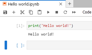
A common issue encountered by new Python optimization modellers is setting up a Python environment. There are many libraries that can be used, and some – like Pyomo – require solvers to be installed separately. Getting everything working can be tricky and frustrating.
So, in this article we'll describe the steps we used to set up a new virtual environment, including Python, Jupyter Lab, several optimization modelling libraries, and a selection of solvers. We'll use this environment for subsequent blog articles about building and solving optimization models in Python.
We hope this article helps you create a working Python environment that enables you to replicate our models and build your own models. Note that we are using 64-bit Windows 10, so everything we do is in that context. If you are using a different operating system, then you'll need to adapt the instructions accordingly.
3 June 2022

We're expanding the scope of this blog to include optimization modelling using Python.
Python is a popular programming language for many data science applications, including optimization modelling. A key feature of Python is the availability of many packages for building and solving optimization models, including:
- CVXPY. Modeling language for convex optimization problems.
- Gekko. Modelling language for machine learning and optimization.
- OR-Tools. General purpose linear, mixed integer, and constraint programming, plus specific tools for vehicle routing and graph algorithms.
- PuLP. Optimization modelling language written in Python.
- Pyomo. Optimization modelling language with a diverse set of optimization capabilities.
- Python-MIP. Collection of tools for the modelling and solution of mixed integer linear programs.
- SciPy. General purpose numerical and scientific computing library.
These tools provide access to a variety of solvers, which help us solve a wide range of problem types. In addition to the solvers built into some of the packages, we'll also use:
- Bonmin. A solver for general mixed integer non-linear programs.
- CBC. A linear and mixed integer program solver.
- Couenne. A solver that aims to find global optima of non-convex mixed integer non-linear programs.
- GLPK. Package for solving large-scale linear and mixed integer programs.
- Ipopt. Package for large-scale non-linear optimization.
- NEOS Server. Internet-based service that provides remote access to many solvers.
- Octeract. A global mixed integer non-linear solver.
As discussed in our article Optimization in Excel vs Python, the choice of optimization tool depends on the circumstances, including the model's features and the modellers' and users' familiarity with the tools. As optimization tools, Excel and Python both have advantages and disadvantages. By expanding our blog's scope to include Python tools, we're looking to enable you to use the approach that works best in your situation.
We'll focus on free and open-source packages and solvers, though the concepts can also be applied to commercial software like CPLEX and Gurobi.
In our next article, we'll step through the process of setting up an environment for Python modelling. In subsequent articles, we'll explore a variety of Python optimization packages, sometimes contrasting a Python model implementation with an Excel implementation.
13 May 2022
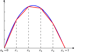
In the real world, we often encounter non-linear relationships in the systems we're modelling. But non-linearities can be difficult to model and even more difficult to solve to optimality.
The recently-published paper "Transformation and linearization techniques in optimization: A state-of-the-art survey" presents a detailed description of transformations and linearizations for a variety of non-linear relationships.
According to the paper's abstract:
To formulate a real-world optimization problem, it is sometimes necessary to adopt a set of non-linear terms in the mathematical formulation to capture specific operational characteristics of that decision problem. However, the use of non-linear terms generally increases computational complexity of the optimization model and the computational time required to solve it.
This motivates the scientific community to develop efficient transformation and linearization approaches for the optimization models that have non-linear terms. Such transformations and linearizations are expected to decrease the computational complexity of the original non-linear optimization models and, ultimately, facilitate decision making.
Asghari et al. (2022). "Transformation and linearization techniques in optimization: A state-of-the-art survey"
The transformation and linearization techniques described in the paper include:
- Multiplication of binary variables.
- Multiplication of binary and continuous variables.
- Multiplication of continuous variables.
- Maximum/minimum operators.
- Absolute value function.
- Floor and ceiling functions.
- Square root function.
- Multiple breakpoint function.
- Piecewise linear approximating functions.
- Log-linearization via Taylor series approximation.
- A new technique for linearizing square root terms by means of transformation.
The detailed descriptions in this paper make a good complement to the booklet MIP formulations and linearizations that we've mentioned previously.
Download the full paper: Transformation and linearization techniques in optimization: A state-of-the-art survey ![]()
If you need help transforming your non-linear model into a linear model, then please contact us.
12 April 2022

In Logic conditions as constraints - Part 1 we introduced a technique for converting a broad class of logic conditions into constraints. While that technique is effective, it can be difficult to apply.
In this article, we present an alternative technique specifically designed to improve the proficiency of students learning to formulate models.
That is, we use two techniques for converting logic conditions into constraints:
- Decomposition and Translation (D&T). This technique is described in the paper "Teaching use of binary variables in integer linear programs: Formulating logical conditions".
- Conjunctive Normal Form (CNF). We described the CNF technique in Part 1.
After describing the D&T technique, we focus on replicating the paper's examples, applying both the D&T and the CNF techniques to illustrate how each technique can be applied to a variety of logic condition formulation situations.
3 April 2022

When formulating a model, we often have a situation described in terms of logic conditions where something implies something else. For example:
- If this happens, then we must do that.
- If this and that happen, then we can't do some other thing.
- We can do some or all of these things, but only if that other thing happens.
However, mathematical programming models cannot represent logic conditions directly. Therefore, we need to translate the conditions, known as "implications", into a set of constraints that represent the logic.
This article describes a technique for converting a logical implication into an equivalent set of constraints. Along the way, we'll dabble in applying some formal logic notation, define rules for manipulating formal logical implications, have a brief look at Conjunctive Normal Form (CNF), and learn how to convert CNF into constraints.
Part 2 describes an alternative representation of this technique, specifically designed to improve the proficiency of students learning to formulate models.
7 March 2022
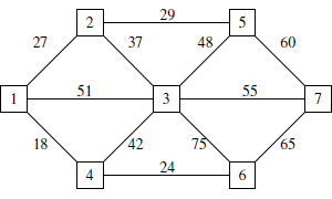
Attached is a free, 681 page textbook: Decision Modeling. The textbook is written by David M. Tulett, Associate Professor in the Faculty of Business Administration at Memorial University in Canada.
Topics covered by the textbook include: optimization of linear, integer, and nonlinear models, as well as the use of decision trees. Both Excel Solver and LINGO are used extensively to build and solve the many example models.
According to the Introduction:
Decision Modeling involves the creation of mathematical models which represent problems faced by business management. To a lesser extent, it also involves numerically solving these models. ...
If there's a difficulty with this subject, it's probably not the mathematics. Instead, the difficulty is likely to be the building of the model which the mathematics seeks to solve. The important thing is always going from a problem description to a model for the problem.
Tulett, D. M. (2022). "Decision Modeling"
Download the full textbook as a PDF (version 3.0.4, 3 March 2022): Decision Modeling ![]()
Updates for the textbook are available from Linney, Memorial University's Centre for Innovation in Teaching and Learning (CITL).
5 March 2022
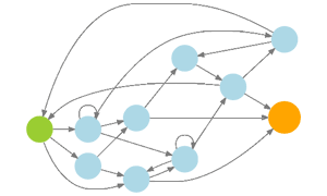
Professor Rubin recently posted an article about finding all solutions to a network model: Finding almost all paths. The article mentions two techniques that we explored in our article Taking a dip in the MIP solution pool. Specifically, Professor Rubin says:
To find all solutions, one possible approach is to solve whatever MIP model you choose, then add a "no-good" constraint that eliminates the solution just found (and only that one) and solve again, until eventually the aggregation of "no-good" constraints makes the model infeasible. What I did instead was to use the "populate" command in CPLEX, which accumulates a pool of solutions.
An issue with the CPLEX solution pool is that it isn't guaranteed to find all optimal solutions. So, the Professor also describes a brute force method to find all solutions. The article presents analysis that demonstrates that the brute force performs better in this case – that is, the brute force method is both faster and more reliably finds all solutions.
Although clever solvers are often the best method we have, it is good to remember that brute force can be a useful – and sometimes efficient – method for solving a problem. We used a brute force method for the situation described in our article Job sequencing to minimize completion time. In that situation, brute force enumeration was very effective for small data sets, though it quickly became impractical for large data sets.
In summary, we can extend our list of techniques for finding all solutions to include:
- CPLEX solution pool.
- Eliminate known solutions.
- Brute force enumeration.
If you know of any other methods for finding all (or almost all) solutions to an optimization problem, or you want help with your own models, then please contact us.
21 February 2022

We're frequently asked questions like: "How many other optimal solutions exist?" and "How do I find those solutions?". Often these questions are prompted by our mentioning that most models have alternative optima – that is, optimal solutions with the same objective function value, but different variable values.
Although a model may have a unique optimal solution, models with integer/binary variables typically have multiple optimal solutions, and continuous linear models may have an infinite number of alternative optimal solutions. The likely existence of multiple alternative optima is why we usually say "an optimal solution", rather than saying "the optimal solution".
Sometimes people also ask, "How do I find solutions that are almost optimal?". This question typically indicates that the decision maker may accept a sub-optimal solution (or an alternative optimal solution) that is "better" according to some criteria that aren't captured by the model design. Of course, we should look at incorporating the unspecified criteria within the model, but sometimes that is difficult or even impossible. In any case, exploring the solution space around the optimal solution is an important part of the modelling process.
This article describes methods for finding alternative optima and solutions that are almost optimal. Specifically, we explore the CPLEX "solution pool" feature, which NEOS Server has recently made available through their online portal.
29 January 2022
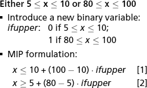
When formulating a model, many of the problems we encounter involve non-linear formulae. For example, a fixed cost is incurred only if a facility is built, or a variable can take values only in the ranges 5 to 10 or 80 to 100.
Optimization models work best when the objective function and constraints are all linear. In some situations, it is possible to reformulate a model to linearize the non-linear parts. The techniques for linearizing non-linear formulae can make the difference between a model being viable or not.
FICO Xpress Optimization have written a booklet that describes a variety of useful mixed-integer programming (MIP) formulations and linearizations, including:
- Binary variable logical conditions.
- Minimum, maximum, and absolute value of binary variables.
- Multiplication of variables.
- Variables with disjunctions.
- Batch sizes.
- Minimum activity level.
The booklet is available at: MIP formulations and linearizations.
